This is a self publication of my graduate thesis in a blog-style format. I hope to make my research more accessible to the public and future research. The text within is unchanged, and only formatting and small grammatical mistakes have been altered. The original ProQuest version can be found here.

I hope you find my research interesting, and enjoy this insight into our ecological past.

Willow Austin

---

Assessing Selection Bias in General Land Office Vegetation Data and Its Implications for Ecological Modeling in the Ouachita Mountains

by

Willow Harper

A thesis presented to the Department of Geography
and the Graduate School of the University of Central Arkansas
in partial fulfillment of the requirements for the degree of

Master
in
Geographic Information Systems

Conway, Arkansas
August 2023

ABSTRACT

Shortleaf pine (Pinus echinata) and oak (Quercus spp.) woodlands in Arkansas are in decline due to the removal of frequent, low intensity wildfire disturbances that maintained their unique composition and structure. They are a focus of conservation and restoration in the state. However, little is known of the historical finer-scale distribution of these fire-adapted habitats in Arkansas’s Ouachita Mountain ecoregion (OME). General Land Office (GLO) surveys are a resource for detailed historical vegetation data that is often used to track changes in vegetation over time, or reconstruct early settlement period forest distribution, density, and composition. However, these surveys are not free from selection species and size biases introduced by individual surveyor preferences or by the surveyor instructions themselves. It is necessary to evaluate the unique selection biases present in GLO surveys, as bias could influence reconstructions of historical vegetation. Much of the GLO survey data for Arkansas’s OME had not been digitized or analyzed prior to this study, and a study examining GLO survey biases in the OME of this scale had not been conducted previously.

This study’s objectives were to analyze the potential species and size selection bias in GLO bearing tree (BT), line tree (LT), and line description (LD) records for Arkansas’s Ouachita Mountain ecoregion and provide recommendations for using these records for historical vegetation reconstructions given the observed bias present. Location and species information for BTs, LTs, and LDs were extracted from GLO survey note scans using optical character recognition (OCR) software, processed using R scripts, and mapped using ArcGIS Pro 2.8.3. Evidence of species and size selection bias was found within GLO surveys conducted in Arkansas’s OME. While there were no significant differences in species mean relative distance across the entire study area, James Trimble’s pine BTs had significantly greater mean relative distance than all other species in his surveys, indicating pine was Trimble’s preferred species for BTs. Size bias differed between the types of vegetation records recorded. On the study area scale, ash, dogwood, and elm BTs were significantly larger than LTs of the same species, indicating bias towards larger individuals of those species in BT records overall. On the scale of individual surveyors, species in Allen Martin and J.E. Graham BTs records and species in James Trimble’s LT records were biased towards larger diameter trees. Individual surveyor species and size bias was masked when analyzing all surveyor records collectively.

---

TABLE OF CONTENTS

1. ABSTRACT
2. TABLE OF CONTENTS
   1. LIST OF ABBREVIATIONS
3. CHAPTER 1: INTRODUCTION
4. CHAPTER II: REVIEW OF LITERATURE
   1. The General Land Office and Public Land Survey System
   2. Assessing Selection Bias in GLO Surveys
   3. Pre-Settlement Vegetation Reconstructions
5. CHAPTER III: METHODOLOGY
   1. Study Area
   2. Data Collection and Processing
      1. PLSS Data
      2. GLO Survey Data
      3. Analysis of Bias in Tree Records
6. CHAPTER IV: RESULTS
   1. Survey Bias in Arkansas’s OME
      1. Historical Context of Survey Collection
      2. Distance Bias in Bearing Tree Records
   2. Differences in Bias by Record Type
      1. Size Bias in Bearing & Line Tree Records
      2. Differences in Species Selection
7. CHAPTER V: DISCUSSION
   1. Survey Bias in Arkansas’s OME
   2. Differences in Bias by Record Type
   3. Differences in Bias by Surveyor
   4. Summary of Species and Size Selection Biases
   5. Recommendations for the Use of GLO Surveys Considering Bias
      1. Forest Composition
      2. Forest Density
      3. Species Diameter Distributions
      4. Species-site Relationships
8. CHAPTER VI: CONCLUSION
9. REFERENCES

LIST OF ABBREVIATIONS

BT – Bearing Tree

FIA – Forest Inventory and Analysis

GLO – General Land Office

LT – Line Tree

LD – Line Description

OCR – Optical Character Recognition

OME – Ouachita Mountain Ecoregion

ONF – Ouachita National Forest

PLSS – Public Land Survey System

SDM – Species Distribution Model

---

CHAPTER 1: INTRODUCTION

The forests of the southeastern United States have changed dramatically in distribution, composition, and structure since the arrival of Euro-American settlers (Hedrick et al. 2007; Nowacki & Abrams, 2008; Strausberg & Hough, 1997). Logging and the clearing of forests for agriculture by settlers fragmented forest ecosystems and eventually led to the removal of almost all old-growth vegetation from the southeast’s forests. Later in the late 1920s and early 1930s, a period of fire suppression supported by government policy began. This prevented the fire-adapted forest ecosystems of the southeast from experiencing the frequent, low to medium intensity fire that maintained their unique composition and structure. These factors all contributed to the significant changes to the distribution, composition, and structure of forest ecosystems in the southeastern United States. These changes have meant the loss of habitat for a number of plant, bird, reptile, and mammal species that relied on fire-adapted forest ecosystems, resulting in many of these species becoming threatened, endangered, or extinct. Natural resource managers are attempting to restore these forests to their historical composition, prior to Euro-American settlement, to prevent further habitat loss for these species. 

Managers often do not know for certain the exact distribution, species composition, average tree size, or the range of densities of the historical forest ecosystems they are trying to manage for. Historical records of vegetation can provide this information to inform landscape management efforts (Bolliger et al. 2004). General Land Office (GLO) surveys are a commonly used source of historical vegetation data and are one of the oldest and most detailed accounts of pre- and early period settlement vegetation in the United States (Bragg, 2004a; Foti & Glenn, 1991; Manies & Mladenoff, 2000; Wang, 2005). GLO survey data is often used as a baseline for comparison with modern vegetation or used to inform models of pre-settlement forest distribution, density, and composition (Batek et al. 1999; Foti & Glenn, 1991; Hanberry et al., 2012; Tulowiecki, 2014; Wang, 2005). 

However, GLO surveys can contain species and size biases that would influence the reconstruction of historical vegetation. GLO surveys were intended to quickly partition the landscape into plots for distribution to Euro-American settlers and not designed as an ecological survey (Bragg, 2004a; Smith, 2012; Wang, 2005). The deputy surveyors and their crews were not formally trained botanists or foresters, and some official survey instructions advised surveyors to avoid smaller trees (Bragg, 2004a; Smith, 2012; White, 1983). Surveyors also likely had preferences for tree species that were easier to blaze or seen as long-living, hardy species (Bourdo, 1956; Grimm, 1984; Schulte & Mladenoff, 2001).  This likely introduced species and size biases in survey records that differs spatially, by deputy surveyor, and by the type of vegetation records recorded, creating a potentially skewed view of pre-settlement vegetation (Batek et al. 1999; Liu et al. 2011; Tulowiecki, 2014; Williams & Baker, 2010). It is necessary to evaluate the unique surveying biases present in GLO surveys, as bias could influence reconstructions of historical forest composition, density, and basal area.

This study’s objectives are to analyze potential species and size bias in GLO bearing tree, line tree, and line description records for Arkansas’s Ouachita Mountain ecoregion (OME) and provide recommendations for using these records for historical vegetation reconstructions given the observed bias. These objectives are assessed through the following research questions: 1) Is there evidence of  bias within General Land Office surveys conducted in Arkansas’s OME? 2) Does this bias differ between the types of vegetation records recorded by surveyors? and 3) Does this bias differ between the individual surveyors who created these survey records? Evidence of species and size selection biases were found in the OME’s GLO surveys, and these biases differed by record type and by surveyor. Surveyor instructions concerning species and size selection and species and size preferences by individual surveyors likely introduced bias to GLO surveys recorded in Arkansas’s OME (Bourdo, 1956; Bragg & Web, 2014; Kronenfeld, 2015; Smith, 2012; White, 1984). It is also likely differences in surveying instructions between record types influenced the introduction of species and size biases to each record type (Larsen et al., 2015; Liu et al., 2011; Tulowiecki, 2014; White, 1984). While species and size biases were found to be present, the influence was minimal on the dominant tree species of the OME’s historical forests. However, species and size selection biases were strongest in species that comprised a smaller percentage of overall forest composition. This could still influence reconstructions made with the GLO survey data and landscape management decision based on those historical vegetation reconstructions. This assessment of bias in the region and the digitized survey records produced by this study could help inform ecosystem conservation and restoration efforts in the OME.

CHAPTER II: REVIEW OF LITERATURE

The General Land Office and Public Land Survey System

The Land Ordinance of 1785 required the surveying of federal lands before they could be distributed for settlement (Bragg, 2004a; Smith, 2012). Later in 1812, The General Land Office (GLO) was established to oversee the surveying of the United States’ public domain, so public lands could quickly be made available as payment for soldiers who would fight in the War of 1812. The land surveys recorded by the GLO are one of the oldest and most detailed accounts of pre-settlement vegetation in the United States (Bragg, 2004a; Foti & Glenn, 1991; Manies & Mladenoff, 2000; Wang, 2005). The work of the GLO shaped the way the United States was settled and the progress of westward expansion during the 19^th century.

In 1803, at the time of the Louisiana Purchase, it is estimated that roughly five hundred Euro-Americans inhabited the lands that would become the state of Arkansas, and most were settled around the White River and the Arkansas Louisiana border (Smith, 2012). Surveying progress in Arkansas was slow for most of the early to mid-1800s, greatly delaying the settlement of Arkansas’s lands. Less than half of Arkansas was surveyed by 1837, twenty-six years after legislation was passed ordering the area be surveyed and sixteen years after Arkansas was put into an independent surveying district to expedite surveying of the state. Surveying of public lands in Arkansas was not finished until 1859. Although progress was slow, the land divisions implemented by the GLO is still used to determine property boundaries in Arkansas and in a majority of the United States.

GLO surveys used the Public Land Survey System (PLSS), created by the Land Ordinance of 1785 to standardize repeatable surveying procedures and to replace the metes and bounds system with a rectangular survey (Bragg, 2004a; Smith, 2012; Wang, 2005). The PLSS divides land into approximately 6-mile by 6-mile parcels with north-south range lines and east-west township lines. Each parcel is called a township and is labeled with a township and range number and cardinal direction according to its position relative to an established meridian and baseline (e.g., T1S R28W). Townships are further subdivided into 36 1-mile square sections, each containing roughly 640 acres, and are labeled 1 to 36. Each section only has two section lines associated with it: the eastern boundary line and the southern boundary line. GLO surveys conducted in Arkansas all reference the 5th principal meridian and baseline, established in 1815 by deputy surveyors Prospect K. Robbins and Joseph C. Brown (Bragg, 2004a; Smith, 2012). 

William Rector, the principal deputy surveyor for the Louisiana territory in 1815, hired Robbins and Brown to conduct the initial baseline and meridian surveys. He would also hire other deputy surveyors to mark townships and survey specific areas outlined in their contract (Bragg, 2004a; Smith, 2012). Deputy surveyors were responsible for locally recruiting their own survey crew. Crews would typically consist of a campkeeper, two chainmen, and an axeman. The campkeeper was responsible for tending to camp and preparing meals, while the chainmen and axeman would work with the deputy surveyor to conduct the survey itself. Chainmen would carry and help handle the measurement chain and other equipment, and the axeman would clear a line of sight for the deputy surveyor to ensure the chain was level. The deputy surveyor would also rely upon their crew to help them identify the species of trees if they were unable to determine the species themselves.

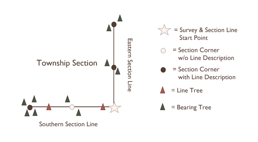
Deputy surveyors would start a survey record by noting what township and section line they were surveying and their heading along that line (e.g., West along the South side of Section 36 Township 1 South Range 28 West) (Bragg, 2004a; White, 1983). They would record the species and diameter of trees that intersected the surveyed section line directly, called line trees (LTs) (Fig. 1). Natural features, such streams, bodies of water, mountain peaks, bluffs, and prairies, would be recorded when they crossed the survey line or were near the line. Human-made features, such as trails, roads, farms, and fields, would also be recorded when they crossed or neared the survey line. Every half-mile the deputy surveyor would set a section corner post. Two to four of the closest trees to the post, called witness or bearing trees (BTs), would have their species, diameter, bearing, and distance from the section corner recorded (Fig. 1). Each section line has two section corners associated with it, and each bearing tree is only associated with one section corner. At these section corners deputy surveyors would also often record the condition of the land and its suitability for cultivation, what timber was present, and the composition of the undergrowth they saw along the line until they reached the section corner. The lists of tree species recorded in these descriptions are called species lists or line descriptions (LDs) (Fig. 1). Some survey records lack these LDs completely for the official survey boundaries, and others only record the condition of the land for cultivation. The distance of features on the survey line were most commonly measured from where the eastern and southern survey lines of a section meet, referred to this this study as the survey start point. Some resurveys of southern lines would have an eastern heading and start from the opposite end of the survey line.

These surveys were conducted by surveyors who were typically well educated with formal land surveying training (Bragg, 2004a; Bragg & Web, 2014; Smith, 2012). The men given deputy surveyor contracts were often reputable, well respected with local renown. The position came with prestige and political power, and it was common for them to seek political office after GLO contracts were completed. Some deputy surveyors were less than reputable, however, and used their position to identify valuable tracts of land for personal gain. Corruption and nepotism were common in the combined Arkansas, Missouri, and Illinois survey district. During William Rectors’ appointment as principal deputy surveyor for the district from 1813 to 1824, Rector’s friends and members of the Rector, Conway, and Sevier families were prioritized for deputy surveyor contracts (Bragg & Web, 2014; Smith, 2012). Not all of them were well suited to the job, such as Charles Pelham. Pelham submitted survey records of over 200 townships in northern Arkansas from 1821 to 1843, most of which were later found to be entirely falsified. Deputy surveyors sent their completed field notes to their regional GLO office for approval. Office clerks were able to check for obvious errors like missing or transposed measurements. However, without being able to go out into the field themselves to verify the survey’s accuracy, office clerks were unable to identify fraudulent surveys themselves. Fraudulent or very poor surveys were typically identified much later by landowners or other deputy surveyors attempting to find survey lines based on the recorded bearing trees.

Initially the GLO pushed for land to be surveyed quickly, prioritizing the division of land over perfect surveying in order to get land allotments to settlers as soon as possible (Bragg & Web, 2014; Smith, 2012). Deputy surveyors also had economic pressure to complete surveys quickly, as they were paid a rate based on the number of miles completed. Errors were perpetuated as surveying progressed, since PLSS-based surveys reference previous work. Since property boundaries rely on the surveyed divisions, errors in line measurements had to be kept once established to avoid widespread disputes over property boundaries. The Fifth Principal Meridian, which is referenced by all PLSS surveys in Arkansas, contains measurement errors ranging from 30 meters to 80 meters (Bragg & Web, 2014). Some of this error could be attributed to the surveying instructions, which did not require that surveyors reference redundant measurements to check their work. The PLSS required that sections be one mile and further subdivisions be a fraction of a mile. However, until 1843 survey instructions did not set rules for how far the surveyor’s measurements could deviate from these divisions. 

Deputy surveyors and their crews were not formally trained botanists or foresters (Bragg, 2004a; Smith, 2012).  The locally hired survey crew were likely more familiar with local vegetation than the non-local deputy surveyor. Common names were used to record tree species in GLO surveys, often lumping together multiple species under the same common name. For example, hickory (Carya sp.) species are rarely further described as ‘black hickory’ or ‘white hickory’ and instead any hickory species is just referred to as ‘hickory’ in the survey notes. Sometimes the more specific common name can refer to multiple species. The primary example in Ouachita Mountain surveys is ‘black oak’, which refers to black oaks (Quercus velutina) but it possibly could have been used for southern red oak (Q. falcata), Shumard oak (Q. shumardii), or northern red oak (Q. rubra) by some deputy surveyors (Foti & Glenn, 1991). Sometimes multiple common names were used to refer to the same species, such as ‘spanish oak’ and ‘red oak’ likely both referring to southern red oak (Foti, 2022; Foti & Glenn, 1991).

As a survey intended for the subdivision of land parcels and not as an ecological inventory, GLO surveys have species and size bias introduced through survey instructions and through surveyor preferences. Instructions tended to recommend that surveyors avoid selecting small tees to serve as BTs, as smaller trees would be more likely to be killed and would be difficult to see from a distance (Bragg, 2004a; White, 1983). BT selection rules were expanded upon in 1831, when the GLO recommended the surveying larger, smoothed barked species to serve as BTs in order for blazing more apparent (Bragg, 2004a; Larsen et al., 2015; White, 1983). Individual surveyor preferences also introduced species and size bias in BT selection. Species may have been preferentially selected as BTs if they were easier to blaze (Bourdo, 1956), thought to indicate land suited for agriculture (Lutz, 1930), were valuable timber species (Bragg, 2004a), or species that were seen hardy or long-lived (Grimm, 1984; Schulte & Mladenoff, 2001). Instructions did not require the survey of LTs or provide recommendations on tree size or species, and it’s often assumed that LT records are less biased than BTs (Batek et al., 1999; Liu et al., 2011). LDs were not required to be recorded until 1815, and only started requiring that timber be ordered in the description by prevalence in 1833 (Larsen et al., 2015; White, 1983). Survey instructions given to deputy surveyors were also not completely standardized until 1855 (Larsen et al., 2015; Liu et al., 2011; White, 1983).

There have been three previous GLO studies in Arkansas’s Ouachita Mountain ecoregion: (Bragg, 2004b; Foti & Glenn, 1991; Jawarneh & Julian, 2012). The first is by Foti & Glenn (1991), in which they used historical records and GLO surveys to examine species composition, density, basal area, and distribution for three sites in the northwestern Montgomery County. Pine, post oak, black oak, and white oak were the species most often recorded by surveyors at each site. The distribution of shortleaf pine, white oak, and black oak across aspects and slopes largely matched modern patterns, with shortleaf pine on south-facing aspects and medium slopes, white oak on north and east-facing aspects and a variety of slopes, and black oak on west-facing aspects. Shortleaf pine was also recorded on northwest aspects in several areas. A majority of the undergrowth on all sites was described as “oak bushes”, potential oak regeneration post fire. In some locations on two sites, Bee Mountain and the red-cockaded woodpecker site, undergrowth was recorded as “no undergrowth”. Foti & Glenn (1991) suggest that this indicates there was no woody undergrowth, and the understory was likely composed of grasses instead. They also outlined the probable scientific names for each common name recorded by GLO surveyors. 

The second previous GLO study in Arkansas’s Ouachita Mountain ecoregion was conducted by Bragg (2004b). He reconstructed forest composition through tree species counts for the Lake Winona Research Natural Area in the eastern OME for 1838, 1931, and 1987 to examine patterns of oak dominance. The 1838 and 1931 reconstructions of forest composition were created using GLO township boundary and subdivision survey records for the township encompassing the research area, the original surveys and later resurveys respectively. In the original surveys conducted from 1821 and 1838, white oak, black oak, and pine were the dominant species recorded as bearing and line trees in the township. Bragg (2004b) mentioned the difficulty in knowing how surveyors sampling preferences, and he suggested that hardwoods may have been oversampled compared to shortleaf pine because of how they stood out from the pine overstory (Bourdo, 1956; Bragg, 2003).

The final previous in the ecoregion was done by Jawarneh & Julian (2012). They developed land cover maps for a 100 by 100 km area centered over Little Rock, Arkansas for the years 1857, 1943, and 1975 to compare to the 2006 National Land Cover Database (NLCD) land cover map. The 1857 land cover map was constructed using GLO survey records and plat maps from that year and a 1870s wetlands map.

Assessing Selection Bias in GLO Surveys

There are several methods that have been developed to assess species and size selection bias in historical surveys. Ideally, independent surveys collected during the same period would be used for comparison (Tulowiecki, 2014). In the OME there are no additional surveys for comparison. However, there are a number of methods for assessing bias using only GLO surveys (Bourdo, 1956; Delcourt & Delcourt, 1974; Kronenfeld & Wang, 2007; Kronenfeld 2015). 

Most literature covering the development and testing of methods for quantifying selection biases is done with BT records, as it’s the most commonly used part of GLO surveys (Bouldin, 2008; Bourdo, 1956; Delcourt & Delcourt, 1974; Grimm, 1984; Kronenfeld 2015; Kronenfeld & Wang, 2007; Tulowiecki, 2014; Wang, 2005; Williams & Baker, 2010). Bourdo (1956) argued that species bias in BTs would present as higher mean corner-to-tree distances for species preferred by surveyors, as surveyors would be purposefully selecting the preferred trees located farther from the post instead of the closest trees as instructed. Delcourt & Delcourt (1974) built on Bourdo (1956) and used ANOVA to analyze differences in mean corner-to-tree distances by species. Bourdo (1956) and Delcourt & Delcourt’s (1974) methods rely on an assumption of homogenous forest density, but this assumption is unrealistic for most forests (Bouldin, 2008; Grimm, 1984; Kronenfeld 2015; Kronenfeld & Wang, 2007; Williams & Baker, 2010). Despite the issues with Bourdo (1956) and Delcourt & Delcourt’s (1974) methods, using ANOVA to analyze differences in mean corner-to-tree distance was the main method for quantifying species selection bias in GLO BT records until the early 2000s (Dyer, 2001; Wang, 2005; Weih & Dick, 2008). Kronenfeld & Wang (2007) suggested utilizing mean distance ranks, and Bouldin (2008) suggested applying the original methods at the scale of individual corners, rather than averaging distances across the entire study area, to reduce the analysis’ reliance on assuming forest homogeneity. Kronenfeld (2015) further expanded upon these ideas and developed a relative distance metric that can be analyzed for species bias using Bourdo (1956) and Delcourt & Delcourt’s (1974) methods. The relative distance metric is calculated by dividing the bearing tree’s distance from the section corner by the mean corner-to-tree distance of all BTs at that corner. This allows for the analysis of differences in corner-to-tree distance by species without needing to assume homogeneous forest density, as distances are made relative to each corner post.

Selection biases in line trees have been less explored than BTs. It is often assumed that LT records contain less bias than BTs, as LTs were not subject to the same size and species selection guidelines as BTs (Batek et al., 1999; Liu et al. 2011). A study done by Liu et al. (2011) tested the validity of this assumption by analyzing the differences in the diameter, distance, and species composition of line trees, bearing trees, and meander trees, or tress recorded along the boundaries of streams, using multiple-factor ANOVA with Tukey’s multiple comparisons. Liu et al. (2011) determined that a difference in mean diameter of >10% demonstrated significance given the large number of records and found that LTs as a whole were significantly larger than BTs. The mean diameter of all LT species was larger than BTs, but not all LT species were significantly larger (Liu et al. 2011). This reveals a potential size bias in LT records favoring larger trees, as larger trees are more likely to be intersected by the PLSS grid. Larger, more easily seen trees could have also stood out to surveyors and be seen as a useful marker for finding the survey line. 

As of 2022, there has been no study that has developed methods for quantifying selection biases in LDs (Larsen et al., 2015). However, studies have theorized that LDs should be less biased than BTs, as LDs did not require the direct survey and marking of individual trees and were not subject to the same tree selection rules as BTs (Batek et al., 1999; Larsen et al., 2015; Tulowiecki, 2014). LDs have been used in past studies to determine species abundance (Lutz, 1930; Lorimer, 1977), create pre-settlement vegetation reconstructions (Batek et al., 1999), and to train species distribution models (SDMs) (Tulowiecki, 2014). Larsen et al. (2015) compared relative species abundance between LDs and BTs using both equal weighting and rank weighting models and then tested their relationships with Pearson’s correlation and Root Mean Square Error. They found that BTs and LDs are better related using rank weighted models than equal weighting, supporting the assertion that LDs are meaningfully ranked by prevalence corresponding to relative abundances (Larsen et al., 2015; White, 1983). 

Pre-Settlement Vegetation Reconstructions

Many studies have utilized the vegetation data recorded in GLO survey records to reconstruct pre-settlement vegetation structure (Liu et al, 2011; Manies & Mladenoff, 2000; Wang 2005). These reconstructions can be used as a source of baseline information for habitat restoration efforts and to reveal the historical distribution of now endangered or functionally extinct species (Bolliger et al, 2004; Tulowiecki, 2020; Wang, 2005). The methods for creating these vegetation reconstructions are greatly varied. Many studies have manually transcribed and digitized the survey notes in order to make the recorded bearing and line trees accessible for analysis (Batek et al, 1999; Bolliger et al, 2004; Dyer, 2001; Foti & Glen, 1991; Olsen et al 2006; Wang, 2007). Transcription and digitization has a high time and labor cost, potentially limiting researchers in the size of their study area. One-way researchers have gotten around this issue is to utilize already transcribed survey notes or already digitized records from previous studies, such as Finley (1951) who manually transcribed GLO surveys for the entire state of Wisconsin. Some studies have developed semi-automated methods of digitizing survey records. One example is Weih & Dick (2008), who created ArcView scripts that allowed them to digitize survey records more quickly. One script allowed them to select already digitized section or quarter section posts and to enter the bearing tree distance and bearings to automatically plot bearing trees. The other calculated the bearing of the selected survey line and automatically plot line trees based on entered distances. 

There are a number of different techniques and models used to reconstruct pre-settlement vegetation, and no one method dominates a majority of studies (Batek et al, 1999; Bolliger et al, 2004; Dyer, 2001; Hanberry et al, 2012; He et al, 2007; Jawarneh & Julian, 2012; Maines & Mladenoff, 2000; Olsen et al 2007; Schulte et al, 2002; Tulowiecki et al, 2014; Wang, 2005; Wang, 2007). There are three main reconstruction approaches: those based on bearing tree dominance and forest density, modeling independent of site conditions, and modeling using site conditions to inform predictions. Studies that fall into the first approach base their reconstructions on bearing tree dominance and density for each survey line, typically using the program MWINDOWS for calculation (Bolliger et al, 2004; Schulte et al, 2002). Studies that follow the second approach, modeling without environmental variable influence, typically use indicator kriging or similar spatial interpolation methods (Maines & Mladenoff, 2000; Wang, 2007). Although Maines & Mladenoff (2000) warns against using indicator kriging for areas less than 10⁴ hectares, as it cannot accurately estimate the area occupied by each vegetation type. More recent studies tend to use the third approach, utilizing environmental data to inform their pre-settlement vegetation reconstructions to create species distribution models (SDMs) that predict species presence through environmental variable associations (He et al., 2007; Hanberry et al., 2012; Tulowiecki et al, 2014, Tulowiecki & Larsen, 2015). These studies typically utilize machine learning algorithms such as random forest or generalized boosting.

One study that followed the third approach was conducted by Hanberry et al. (2012), in which SDMs for historical and modern vegetation were created and compared to determine if historical vegetation-site relationships were disrupted in the Missouri Ozarks. Historical vegetation data for this study was BTs from GLO surveys conducted from 1815 to 1850, and modern vegetation data was collected from the USDA Forest Inventory and Analysis (FIA) program surveys (Hanberry et al., 2012). Hanberry et al. (2012) utilized 24 environmental variables, including elevation, slope, transformed aspect, solar radiation, topographic position index, wetness convergence, and 15 soil variables from the Soil Survey Geographic (SSURGO) database. Hanberry et al. (2012) used random forest (Breiman, 2001) as their primary classification modeling technique for all tree species except shortleaf pine (Pinus echinata), for which they used generalized boosting methods to better model the species within a bounded distribution. 

Another study creating SDMs informed by environmental variables was conducted by Tulowiecki (2014), in which he examined LD records and its use for training SDMs compared to typical BT trained SDMs. LDs were mapped as points in the center of the segment they describe with presence and absence of species from the LD record. Environmental variables included mean temperature, compound topographic index, potential evapotranspiration, precipitation, mean solar radiation, and soil drainage, percent clay, percent sand, and pH. Tulowiecki (2014) utilized five algorithms for each SDM: boosted regression trees, generalized additive models, generalized linear models, multivariate adaptive regression splines, and random forests. The results of these algorithms were then combined to create the final SDMs using a formula that increases the influence of better performing single models. Analysis of model performance found that the SDM trained with LD records had significantly greater predictive performance than the BT SDM. Tulowiecki (2014) attributes this to bias in the BT records impacting model performance and differences in sampling between BT and LD records.

CHAPTER III: METHODOLOGY

This study assesses the presence species and size bias within GLO vegetation data within Arkansas’s OME and provides recommendations for using these surveys for historical vegetation reconstructions given the potential bias present. Specifically, is there evidence of selection bias within General Land Office surveys conducted in Arkansas’s Ouachita Mountain ecoregion, and does this bias differ between the types of vegetation records recorded by surveyors? 

There is an established assumption of species and size selection bias discussed by many previous GLO studies, based upon differences in surveying instructions for each record type (Liu et al., 2011; Wang, 2007; Williams & Baker, 2010). This study expands upon the body of literature that tests these assumptions of bias and quantifies bias for bearing tree records, as well as line trees and line descriptions. This study also builds upon previous GLO studies conducted in Arkansas’s OME, as previous studies covered smaller portions of the ecoregion and no previous study has quantified GLO selection biases in Arkansas’s OME (Bragg, 2004b; Foti & Glenn, 1991; Jawarneh & Julian, 2012). Much of the GLO survey data for Arkansas’s OME has not been digitized prior to this study. Additionally, a study examining selection biases in GLO surveys for the OME of this scale has also not been conducted previously. Understanding the species and size selection biases present within GLO surveys for Arkansas’s OME will allow natural resource managers to better understand and apply the historical vegetation data to their landscape conservation and restoration efforts. 

Study Area

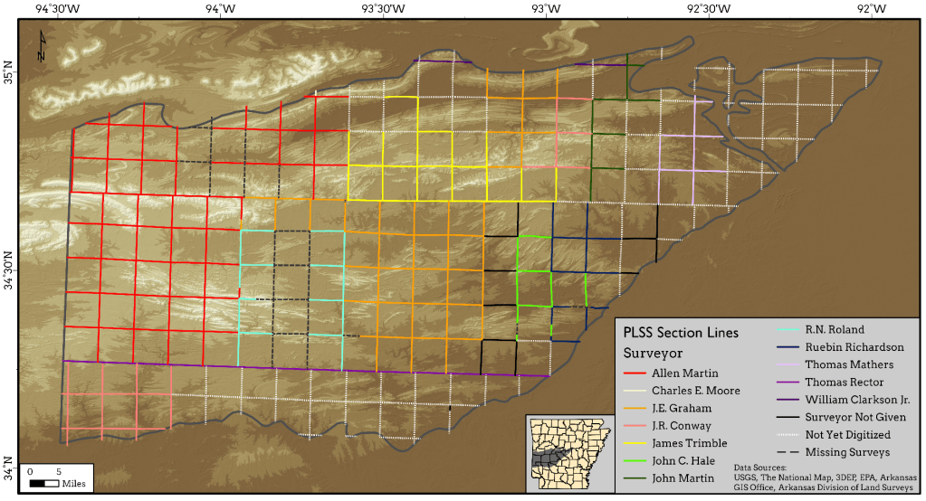
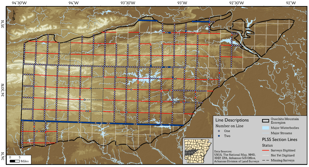
Arkansas’s Ouachita Mountains Level III ecoregion (U.S. EPA, 2010) is the focus area for this study (Fig. 2). This ecoregion covers 16,406 square kilometers across central and western Arkansas. The ecoregion contains 222 PLSS townships and 2,152 township boundary section lines. It covers the entirety of Montgomery, Polk, and Garland counties, and portions of twelve other counties including Clark, Faulkner, Hot Spring, Howard, Lonoke, Perry, Pike, Pulaski, Saline, Scott, Sevier, and Yell counties. In Fig. 2, the section lines in red had their section lines collected, digitized, and mapped. The dashed gray section lines had survey notes that could not be located in Arkansas’s GLO survey archive. The dashed white section lines did not have their survey notes collected, digitized, and mapped by this study. Resources were focused on the collection and digitization of core areas of the ecoregion that best represent the OME as a whole. 1,515 section lines of the total 2,152 section lines had survey notes included in this study. This comprises 70.4% of the total township boundary section lines in Arkansas’s OME. Due to constraints, fringe areas of the OME were not able to have their survey notes digitized for this study.

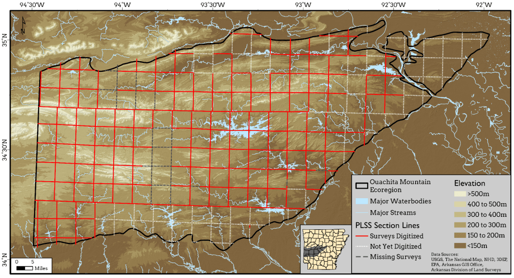
The Ouachita Mountains cover 6.6 million acres over portions of central and western Arkansas and southeastern Oklahoma (Foti & Glenn, 1991; Hedrick et al, 2007; Ouachita Mountains Ecoregional Assessment, 2003). The Ouachitas are an eroded mountain system that formed 280 million years ago in the late Paleozoic period by tectonic activity, creating predominantly east-west running ridges of sandstone and novaculite and valleys of shale. Elevation ranges from 100 meters in the river valleys to 900 meters in the ridges in western Arkansas and southeastern Oklahoma. These differences in elevation expose the peaks and ridgelines to colder winter temperatures and the valleys to cold air drainage. The climate is considered humid subtropical, with hot summers and cool winters. Precipitation is evenly distributed throughout the year, and total yearly precipitation ranges from 1100mm to 1500mm. Soils in the ecoregion are primarily Ultisols, acidic, well-weathered, and moderately well-draining.

Historical descriptions of the Ouachita Mountain region portray ridgelines dominated by pine and oak with open, grassy understories and lowland areas dense with canebrakes, briars, and vines (Dunbar, 1807; Featherstonehaugh, 1844; Nuttall 1821; Schoolcraft 1819). Prior to the arrival of Euro-Americans, the region was inhabited by Native American tribes such as the Caddo (Brooks, 2010). Indigenous people in the eastern United States regularly lit fires to clear understory vegetation, increasing ease of travel, hunting, and agriculture (Abrams et al, 2022; Black et al, 2006; Nowacki & Abrams, 2008). Descriptions of the Ouachita Mountains written by Dunbar (1807), Nuttall (1821), and later Featherstonehaugh (1844) described how both Native Americans and Euro-Americans alike would light fires during the fall and winter. This would thin the forest understory and make travel and hunting easier. It is also thought that land management by Indigenous peoples in the eastern United States selected for oak (Quercus sp.), hickory (Carya sp.), and chestnut (Castanea sp.) tree species and encouraged a mosaicked landscape of fire-adapted vegetation communities of oak savannas, woodlands, and prairies (Abrams et al, 2022; Black et al, 2006). The high frequency of fire disturbance in the pre-settlement period promoted and maintained open oak and shortleaf pine forests in the Ouachitas (Foti & Glenn, 1991; Hedrick et al, 2007). Post-fire regeneration of herbaceous plants would have also provided forage for elk (Cervus elaphus) and bison (Bison bison) that were historically present in the region (Hedrick et al, 2007; Masters, 2006).

During the settlement period, fire frequency and severity increased in forested areas where Euro-Americans were cutting and burning forests to make space for agriculture (Nowacki & Abrams, 2008). This increase in fire led to the ignition of mesic hardwood forests that had rarely burned during the pre-settlement period. However, other areas saw a dramatic decline in fire during the settlement period. In fire-prone landscapes such as grasslands and prairies, Euro-Americans suppressed fire because of the danger to human life and high risk of destruction to structures. Grasslands and prairies were also replaced by cropland and pasturage and fragmented by roads and later by railways. The loss of indigenous ignitions, the Euro-American fire suppression efforts, the conversion of grasslands and prairies to agricultural lands, and landscape fragmentation all contributed to the decline of native grassland and prairie ecosystems during the settlement period. 

Vegetation continued to change from pre-settlement patterns during the post-settlement period, with the large-scale logging of original forests and the government implementation of fire suppression policies (Hedrick et al, 2007; Nowacki & Abrams, 2008). Commercial logging would begin in western Arkansas during the late 1870s and early 1880s (Strausberg & Hough, 1997), and later widespread clear cutting of forests would begin in the early 1910s through the 1940s, removing most forests remaining from the pre-settlement period (Hedrick et al, 2007; Nowacki & Abrams, 2008). The U.S. Forest service began a policy of fire suppression in the 1930s that continued into the 1980s, eliminating the disturbance that maintained many pre-settlement vegetation communities. 

Modern vegetation in the Ouachitas is the result of the replacement of Indigenous fire-based land management practices with Euro-American agricultural land use during the settlement period and later clear cutting and fire suppression during the post-settlement period (Foti & Glenn, 1991; Hedrick et al, 2007; Nowacki & Abrams, 2008). The second-growth forests that grew after clear cutting and the start of fire suppression are denser, with the understory primarily consisting of woody vegetation instead of grasses and forbs. Mesic, fire-sensitive hardwood species, such as red maple (Acer rubrum), have broader distributions now that they are no longer being excluded by fire (Nowacki & Abrams, 2008). Many forests in the Ouachitas have been replaced by timber industry plantations of loblolly pine (Pinus taeda), expanding their distribution in the region (Hedrick et al, 2007). Native bird and mammal species have also been negatively impacted by these shifts in vegetation. The red-cockaded woodpecker (Picoides borealis), once found in abundance in the Ouachitas, is now an endangered species, and elk and bison have become extirpated from the region.

Arkansas’s Ouachita Mountains ecoregion (OME) is ecologically important to the state. It contains many of Arkansas’s threatened species and vegetation communities, which are disappearing due to agricultural land use and fire suppression (Hedrick et al., 2007; U.S. Forest Service 2005, 2017a). There are ongoing conservation and ecosystem restoration efforts in the OME, specifically within the Ouachita National Forest (Hedrick et al., 2007; U.S.F.S., 2005, 2017a, 2017b). Ouachita National Forest (ONF) vegetation management is largely focused on the conservation and restoration of five upland vegetation communities including “Ouachita Shortleaf Pine-Oak Forest”, “Ouachita Shortleaf-Pine Oak Woodland”, “Ouachita Shortleaf Pine-Bluestem”, “West Gulf Coastal Plain Pine-Hardwood Forest”, and “Ouachita Dry-Mesic Oak Forest” (U.S.F.S., 2005, 2017a, 2017b). For pine-oak dominated communities, the desired condition described in the ONF management plan is for 40-65 percent to be shortleaf pine-oak forest, 20-45 percent as shortleaf-pine oak woodland, 7-20 percent as shortleaf pine-bluestem (U.S.F.S. 2005). The full revised forest plan also includes seven other vegetation communities of concern, including “Ouachita Mesic Hardwood Forest”, “Ouachita Montane Oak Forest”, “Ouachita Dry Oak Woodland”, “Ouachita Novaculite Glade and Woodland”, “Central Interior Highlands dry Acidic Glade and Barrens”, “Central Interior Acidic Cliff and Talus”, and “Calcareous Prairie”. Management techniques they employ to maintain several of these communities and to meet their forest composition goals include prescribed burning and both commercial and non-commercial thinning. 

There is a need for pre-settlement vegetation data and reconstructions within Arkansas’s OME to serve as a baseline for restoring historical vegetation composition and structure. Such reconstructions could be compared to current forest conditions and management goals and be used to validate or revise management objectives.

Data Collection and Processing

PLSS Data

PLSS section boundary polygons were downloaded from the Arkansas GIS Office’s data clearinghouse (FGDC Cadastral Subcommittee & Arkansas GIS Office, 2014). These section polygons were converted to line features, and township, range, and section information was assigned to each sections’ eastern and southern boundaries. The length and azimuth of each section line was also calculated and added to the attribute table. The points where each section’s eastern and southern boundaries intersect were also manually digitized and assigned the same township, range, and section information as their associated section. These locations serve as starting coordinates for calculating the locations of survey records, including line trees, bearing trees, and line descriptions. This study only utilizes GLO township boundary surveys, as these were conducted first and capture the oldest picture of vegetation (Smith, 2012; Bragg & Webb, 2014). Subdivision surveys were completed much later than the township boundaries, and the vegetation they recorded was likely more heavily influenced by settlement. Only early surveys of township boundary section lines were collected, digitized, and mapped.

GLO Survey Data

The GLO land survey records used for this study are transcribed copies of the original handwritten notes, created in the 1930s by the Works Progress Administration (Bragg, 2004). These typewritten transcriptions were scanned and archived by the State Lands Office. GLO survey books with records within the study area were identified using the Arkansas Division of Land Survey’s GLO Map 2.3 web map (Arkansas Division of Land Surveys & Arkansas GIS Office, 2022). Each township on the map links to a PDF of its associated survey book, allowing for the quick identification of needed records without manually going through the full GLO survey archive. There are four townships on the map that have no linked survey book. Other townships have a linked survey book, but the pages of that contain the records for that township were not scanned and archived. The coverage of surrounding survey books accounts for some of these areas, but there are still townships lacking survey records. Surveys conducted by known unreputable deputy surveyors, such as Charles H. Pelham, were omitted and replaced by later resurveys if available (Bragg & Web, 2014).

High resolution scans of the transcribed survey books were collected from the Arkansas State Archives after identifying the books needed to cover the Ouachita Mountain ecoregion. The scans were then digitally enhanced to improve the accuracy of optical character recognition (OCR) using batch photo editing software. Contrast between the text and background was increased, and visual noise in the background was reduced as much as possible without reducing the clarity of the text.

ABBYY’s FineReader PDF 15 (2020) OCR tools were used to transcribe the survey notes into Excel spreadsheets in order for the records to be processed digitally. Text recognition was done automatically by the software and then manually checked for errors before outputting the survey book spreadsheet. Township, range, and section label information as well as species names, diameters, bearings, and distances were all checked to ensure accuracy. Output tables included two columns, the first for survey headings and distances along survey lines, and the second for the boundary information and survey records associated with each heading and distance. 

The spreadsheet output by FineReader PDF 15 was then edited in Excel to make later data parsing and calculations in R easier. Five columns were added. The first two additional columns are chain and link distances separated from the combined heading, chains, and links column (Fig. 3). The chain and link columns were then used to calculate distances in both miles and meters. The final additional column is for connecting each record with the survey book it was extracted from. At this stage, survey records for ‘random’ section lines were removed. These were unofficial boundaries temporarily created by surveyors to orient themselves so they could place the ‘true’ or official section line in its intended location. Because these lines were not official property boundaries, the records for random lines did not any contain bearing tree or line tree records. However, surveyors would sometimes include line descriptions for their random lines instead of the true line. These line descriptions were excluded from digitization because they were not recorded on the official section line boundary.

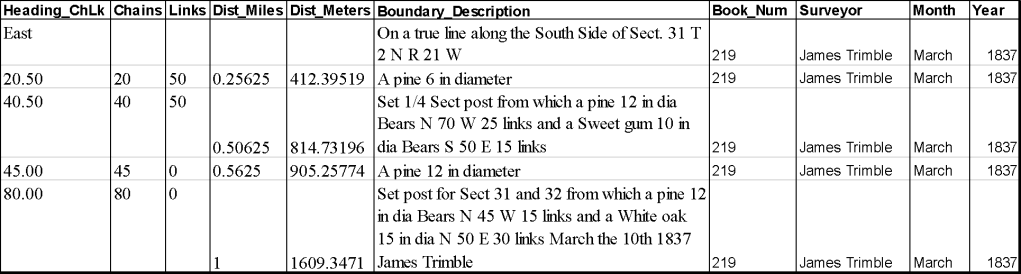
Three scripts in the R programming language (R Development Core Team, 2021) were written to process the edited survey notes spreadsheets. The first script handles data wrangling and basic statistics. It first combines the individual survey book spreadsheets together into one large table. Then it finds and corrects a list of common, consistent OCR errors. These small errors, such as the ‘l’ in links being mistaken for an ‘I’, are misrecognitions that do not impact GLO tree species data accuracy and are quicker to fix with the script than manually. The script then makes species names consistent. For example, records of black oak can be spelled “black oak”, “b oak”, or “b. oak”. The script ensures species names are spelled out and removes any spaces within the name for easier extraction. After fixing these text issues, the script then parses out survey headings, as well as the township, range, and section information recorded at the beginning of each survey entry (Fig. 4). The township, range, and section information is formatted into an ID to connect all records with their associated section. For example, S_Sec36_T2N_R21W would be the ID for the south boundary of section 36 in Township 1 North Range 21 West.

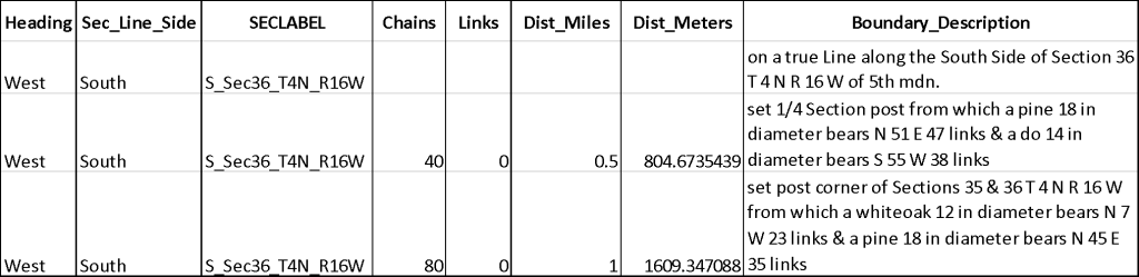
After fixing OCR errors, ensuring consistency in species name spellings, and ensuring every record has associated PLSS location information, the first script then extracts line tree, bearing tree, and line description records into columns within the same table (Fig. 5). Line tree columns include species and diameter in inches, while bearing tree columns include species, diameter in inches, as well as bearing and the distance of the tree from the section post. Line description columns include land, timber, and undergrowth descriptions. These columns will be parsed into separate spreadsheets by record type in the second script.

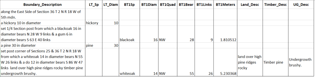
Once the bearing tree, line tree, and line description records have been parsed from the survey records into separate columns, the table is then joined with the attribute tables from the section line and survey start location datasets using the section ID. This associates each record with its section line’s length, azimuth, and the starting location for surveying the section line. This information will later be used by the second script to calculate coordinates for each survey record. Survey records that are not matched to a section line and corner do not fall within the study area and were removed. The final function of the first script is to calculate basic statistics and to create figures, such as counts of species in each record type, average diameter by species, and average distance of bearing trees by species.

The second script uses the recorded distance along the section line, the line’s azimuth in radians, and the section corner coordinates to calculate the coordinates of each record in the NAD 1984 UTM Zone 15N projected coordinate system. These coordinates are the locations of each LT and the locations of BT posts associated with each BT and LD.

     $d * cos( α ) + φ$  (Eq. 1)

     $d * sin(α) + λ$  (Eq. 2)

Northing calculations utilize the formula as seen in (Eq. 1), which has the distance along the section line in meters (d) multiplied by the cosine of the azimuth in radians (α) added to the northing of the section corner (φ). Easting calculations utilize the formula as seen in (Eq. 2), which has the distance along the section line in meters (d) multiplied by the sine of the azimuth in radians (α) added to the easting of the section corner (λ). The second script then partitions the BT, LT, and LD columns into separate tables, retaining their section, township, and range identifying information and the survey text associated with each record. For the LD table, the script calculates description coordinates at the center of the line segment the description covers, following Tulowiecki’s (2014) methods. For sections with two descriptions, one at the quarter section post and one at the section post, the LDs are plotted at the center of each corresponding half of the line. Sections with only one description at the section corner have the LD is plotted at the center of the line. The bearing tree records are still section post points at this stage, and were later partitioned into their own individual locations in the third script.

The individual bearing tree, line tree, and line description records were then plotted in ArcGIS Pro. Some points were off the section line by two to five meters, due to the section line azimuths being an average of a multipart line features. The NEAR tool was used to fix this error in the calculated coordinates, creating new correct easting and northing fields. With the fixed coordinates, the bearing tree records were then run through a third script to partition each bearing tree into its own point using the recorded bearings and distances. 

Analysis of Bias in Tree Records

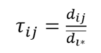
Analysis of bearing tree mean species corner-to-tree distance and mean species relative distance was conducted to determine species bias through significantly greater mean distances. Undertaking both mean species corner-to-tree distance and mean species relative distance also allowed for the comparison of traditional and updated BT distance-based bias analyses. BTs at section corner posts with all identical BT species recorded at that location were excluded from both analyses, as there were no other species for surveyors to preferentially survey (Delcourt & Delcourt, 1974). Relative corner-to-tree distance of bearing trees by species was calculated following methods outlined by Kronenfeld (2015), where the distance from the ith corner to the jth BT at the corner is divided by the mean corner-to-tree distance of all BTs at the ith corner (di*) (Eq. 3).

ANOVA was used to test for any significant differences in mean corner-to-tree distance and mean relative distance amongst all species with greater than 25 recorded individuals. If significant difference in the mean corner-to-tree distance or relative distance was found, post-hoc t-tests assuming unequal variance were used to determine which species mean distance is significantly different from all other species (Delcourt & Delcourt, 1974; Kronenfeld, 2015). Species with a significantly greater mean relative distance were likely more desirable for survey and picked preferentially over closer trees of other species. Species with a significantly greater mean corner-to-tree distance indicates the species were likely more frequently present in less dense forests than other species, rather than indicating the presence of species bias favoring the selection of that species. This is because the analysis of mean corner-to-tree distance relies on an assumption of forest density, including all species, being consistent across the study area to detect species bias rather than natural differences in overall forest density. 

After performing these analyses of BT distance-based species bias for all collected surveys, they were also performed by surveyor to determine differences in individual species selection bias and as a contributor to species bias across the study area. We assessed species bias between the three surveyors who completed surveys of at least 150 sections lines. Previous studies have recommended that analyses and reconstructions be performed on areas comparable in size to the average county (Maines & Mladenoff, 2000; Wang, 2005). However, average county size is subjective and depends on the region of the country. Jenks natural breaks was used to determine the class with the largest areas covered by each surveyor, and greater than 150 section lines was the largest class.

ANOVA was used to test for any significant differences in mean corner-to-tree distance and mean relative distance amongst all species at least 10 recorded individuals after excluding same species section corners. As with the study area wide analyses, post-hoc t-tests assuming unequal variance were utilized if significant difference in the distances was found.

Size bias favoring larger trees was determined by comparing the mean diameter in inches of species in LT and BT records. We followed Liu et al.’s (2011) methods using t-tests assuming unequal variance to compare mean diameters of the record types. We only included species with at least 15 records in both record types. If both sampling methods surveyed forests without size bias, the mean diameter of species in each record type should not be significantly different from one another. If larger trees were selected for either BT or LTs, then the mean diameter would be significantly larger in one record type. After performing the analysis of size bias for all collected surveys, it was also performed by surveyor to determine differences in individual size bias and collective size bias for the study area as a whole. Surveyors who completed surveys of at least 150 section lines were included to ensure enough records for analysis. Species with at least 10 recorded individuals in both record types were included.

Total count of unique species was determined for bearing tree, line tree, and line description records across the study area. The average species richness for townships was calculated for each record type using townships with BT, LT, and LD records for all 12 township boundary sections. Species richness provided insight into the completeness of each of the different tree record types. For example, smaller trees or uncommon trees may have been ignored in the selection of bearing trees or line trees.

CHAPTER IV: RESULTS

Survey Bias in Arkansas’s OME

Historical Context of Survey Collection

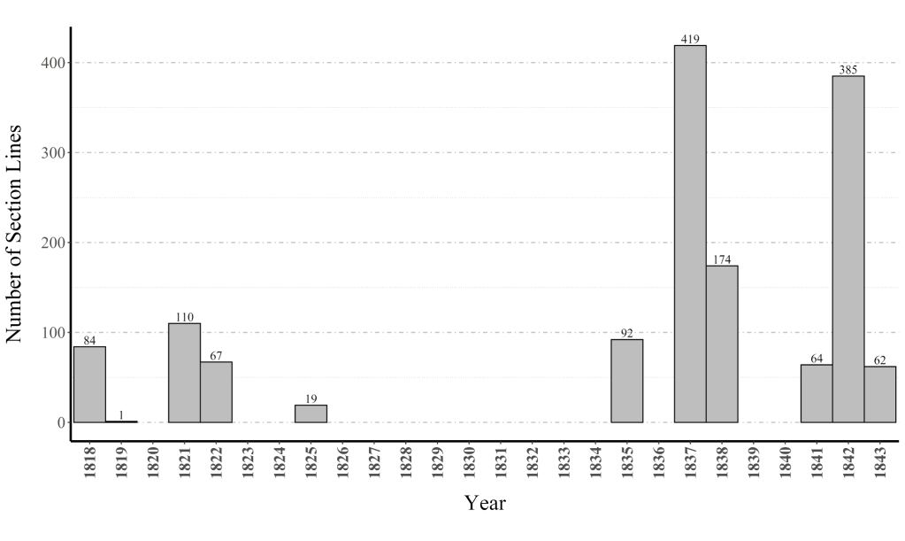
The collected GLO surveys were conducted over a 25-year period from 1818 to 1843, with most section lines being surveyed between 1835 and 1842 (Fig. 6). The median year of survey was 1837. Surveys were first conducted in the southern OME along the PLSS baseline, then generally progressed from northeast to west over time (Fig. 7). The PLSS baseline in the southern OME was surveyed in 1818, and the eastern area of the OME was surveyed in the early 1820s. The central and western areas of the OME were surveyed later in the late 1830s and early 1840s. 37 section lines had no year recorded in their associated survey book. 

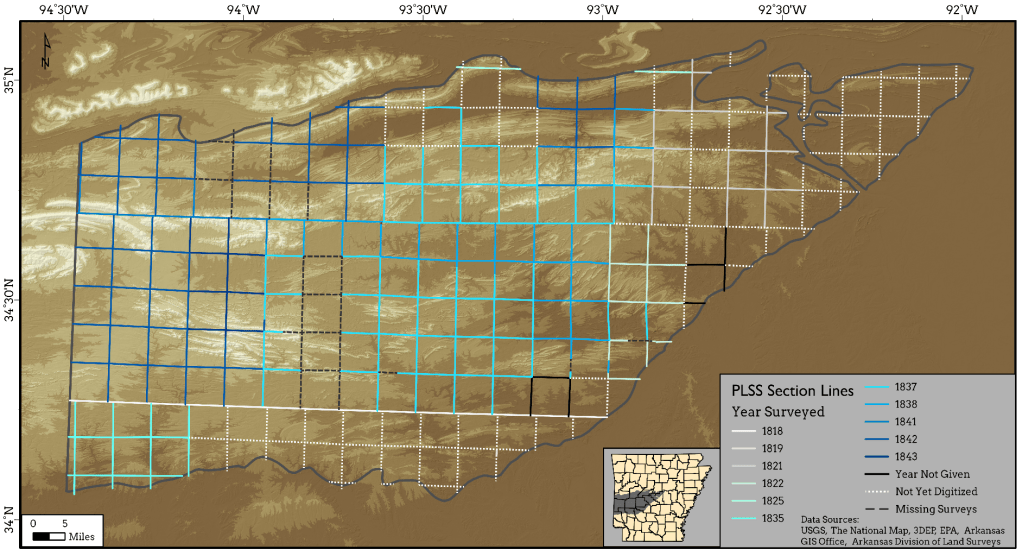
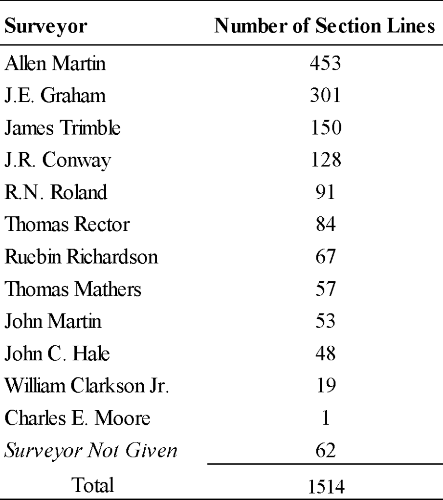
A total of 12 surveyors conducted and recorded the collected surveys covering a total of 1,512 section lines (Table 1). Allen Martin and J.E. Graham surveyed a majority of the collected section lines in the central and western areas of the OME (Fig. 8). Thomas Rector surveyed the PLSS baseline in the southern OME. 62 of the collected section lines had no deputy surveyor name written in their associated survey books.

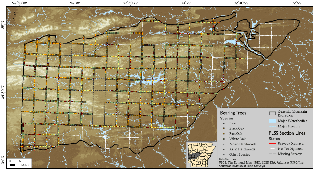
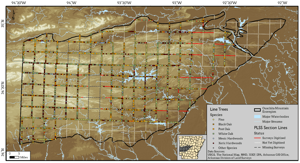
A total of 7,702  records were digitized and mapped from 30 GLO survey books for Arkansas’s OME. The tree records included 5,995 bearing trees (Fig. 9), 3,519 line trees (Fig. 10), and 1,021 line descriptions (Fig. 11). All the digitized and mapped section lines had BTs associated with them, except for a handful of instances where there were no trees to survey as BTs due to an obstacle. Obstacles impassible to surveyors included swamps and instances where the section corner fell in the middle of a river. No line trees were recorded on 102 section lines, as they were not required to be surveyed. The surveyors John Martin (25 section lines), Thomas Mathers (18), Ruebin Richardson (17), and R.N. Roland (16), had the most section lines with no surveyed LTs. Line descriptions for the true section lines were recorded for 974 of the total 1,514. 71.5% of LDs were on eastern section lines, and only 28.5% of LDs were recorded on southern lines. Section lines typically only included one LD. However, surveyors Thomas Rector and William Clarkson Jr. recorded two LDs per section line in a majority of their surveys.

Distance Bias in Bearing Tree Records

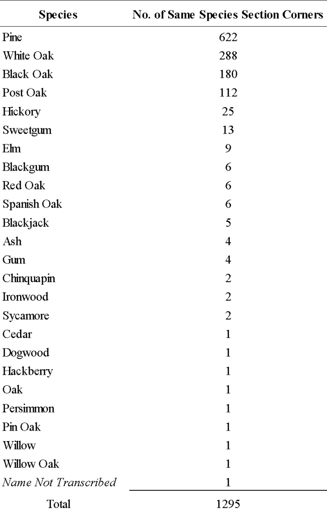
Previous studies examining distance-based species bias in bearing trees have excluded the bearing trees at section corners where all BTs are the same species (Delcourt & Delcourt, 1974; Kronenfeld, 2015). This exclusion is because of the assumption that no other species present at that location, meaning surveyors would have no choice in what species to preferentially survey at those section corners (Delcourt & Delcourt, 1974). Of all 5,995 bearing trees recorded, 2,768 BTs were recorded at these same-species section corners and were removed from mean corner-to-tree distance and mean relative distance analyses. There were 1,295 same-species section corners out of the total 2,930 section corners digitized and mapped (Table 2). 48.0% of same-species section corners recorded all pine, and 46.3% recorded a single oak species. 

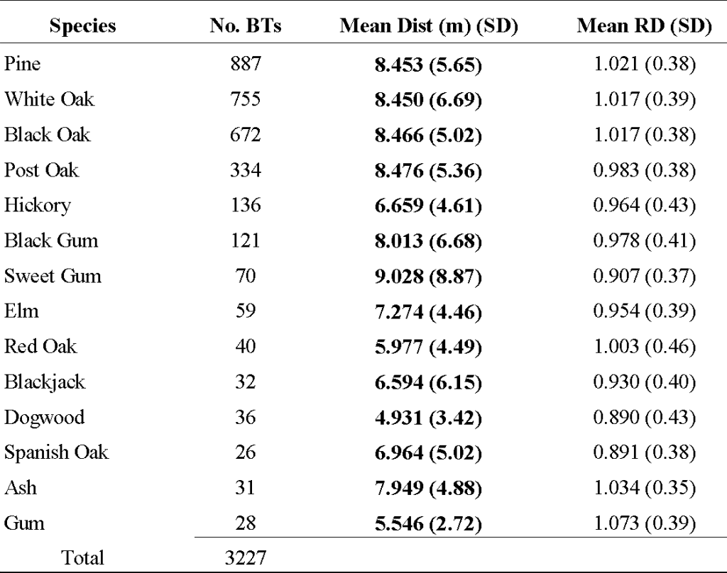
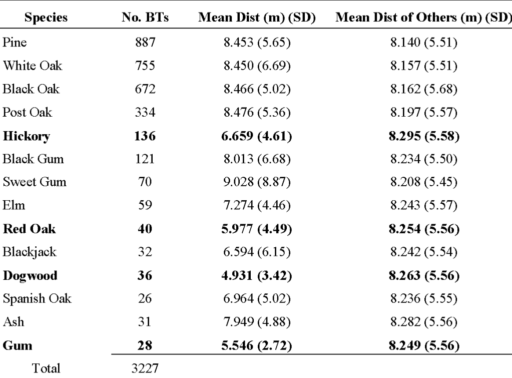
Analysis of bearing tree mean species corner-to-tree distances revealed significant differences in mean corner-to-tree distance between species (ƒ = 3.8, p < 0.001) (Table 3). Post-hoc t-tests assuming unequal variances revealed that hickory (p < 0.001), red oak (p = 0.003), dogwood (p < 0.001), and gum’s (p < 0.001) mean corner-to-tree distance are significantly smaller than all other species (Table 4). The historical forests of the Ouachita Mountains likely varied in density across the ecoregion because of the variability of elevation and the presence of regular fire disturbances during the time period (Dunbar, 1807; Featherstonehaugh, 1884; Foti & Glenn, 1991; Nuttall, 1821). Because the study area does not fit the assumption of homogenous forest density across the study area, the analysis of mean corner-to-tree distance suggests these species were recorded in denser forests overall, rather than being species that were biased against. Sweet gum had the greatest mean corner-to-tree distance at 9.028 meters, while pine, white oak, black, and post oak all had mean distances between 8.450 and 8.476 meters. Hickory, red oak, dogwood, and gum had mean corner-to-tree distances between 6.659 and 4.931 meters. However, analysis of bearing tree mean species relative distance revealed no species with a significantly different mean relative distance (ƒ = 1.5, p = 0.109) (Table 3). Mean relative distances ranged between 0.890 and 1.073, with no extreme deviations from the expected value of 1.

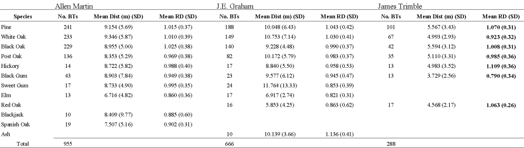
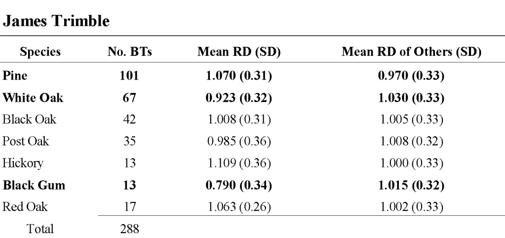
Trends in mean corner-to-tree distance and relative distance by species differ by individual surveyor (Table 5). Allen Martin’s surveys showed no statistically significant difference in mean species corner-to-tree distance (ƒ = 0.7, p = 0.702) or mean species relative distance (ƒ = 0.8, p = 0.643). J.E. Graham’s surveys were similar, with no statistically significant difference in mean species corner-to-tree distance (ƒ = 1.9, p = 0.052) or mean species relative distance (ƒ = 1.4, p = 0.170). However, the analysis of James Trimble’s surveys revealed a significant difference in mean species relative distance (ƒ = 2.7, p = 0.013). Post-hoc t-tests assuming unequal variances revealed pine’s relative distance is significantly larger than all other species in Trimble’s surveys (Table 6). Additionally, white oak and black gum’s relative distance was significantly smaller than all other species. Pine had a relative distance of 1.070, while white oak had a relative distance of 0.923. Black gum had an especially small relative distance of 0.790. This suggests that James Trimble’s surveys contain species bias favoring pine, because he was traveling significantly farther distances, ignoring closer trees, in order to survey pine. The significant differences in mean relative distance by species also suggests Trimble’s surveys contain species bias against white oak and black gum. It is likely that Trimble was only surveying white oak and black gum out of convenience if the species were located close to the section corner and if a more preferred species were not present. While Trimble was not noted in the literature as being an unreputable surveyor, the results of this analysis suggests Trimble’s surveys were influenced by his preferences for species (Bragg & Web, 2014; Smith, 2012).

Differences in Bias by Record Type

Size Bias in Bearing & Line Tree Records

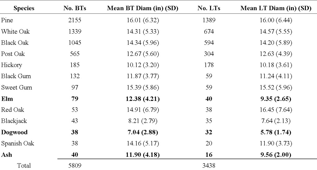
T-test comparisons of mean species diameters in inches between bearing tree and line tree records revealed three species, elm (p < 0.001), dogwood (p = 0.028), and ash (p = 0.007), had significantly larger mean diameters in BT records than LT records (Table 7). Elms recorded by BT records were an average of 3.03 inches larger than elms recorded as LTs. Ash BTs were an average of 2.34 inches larger than ash LTs, and dogwood BTs were an average of 1.26 inches larger than dogwood LTs. Spanish oak BTs were an average of 2.26 inches larger than Spanish oak LTs, but this difference was not found to be significant (p = 0.062). Additionally, Red oak LTs were an average of 1.54 inches larger than red oak BTs, but this difference was also not found to be statistically significant (p = 0.324). The mean diameter of pine, white oak, black oak, post oak, and hickory recorded in both record types were all within 0.2 inches of one another.

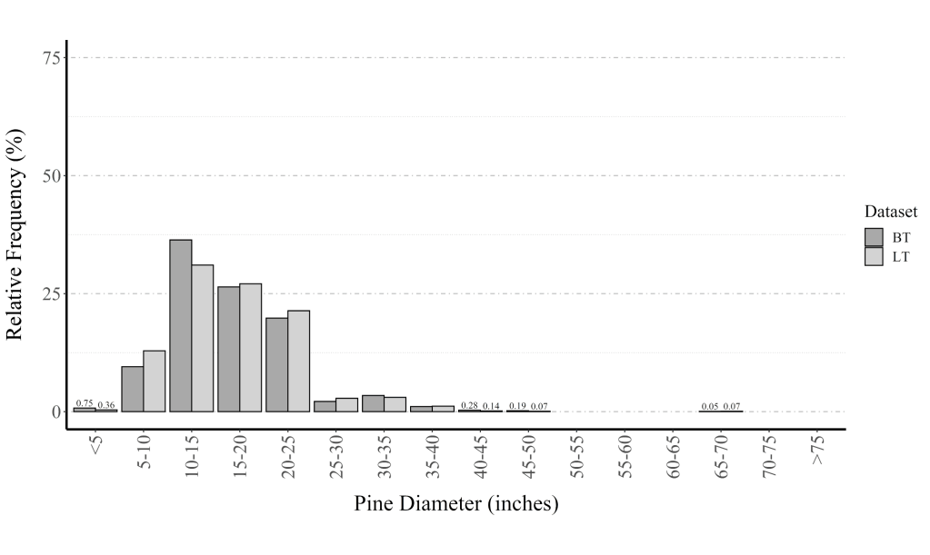
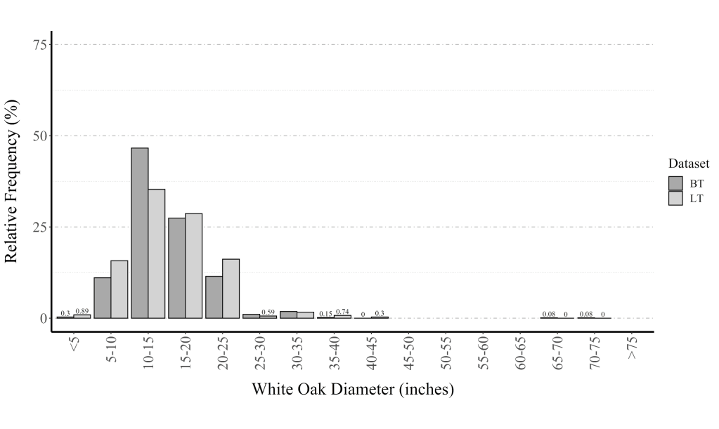
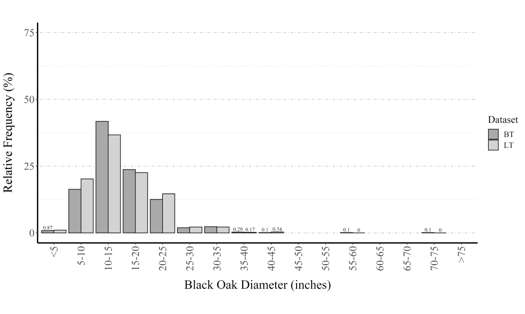
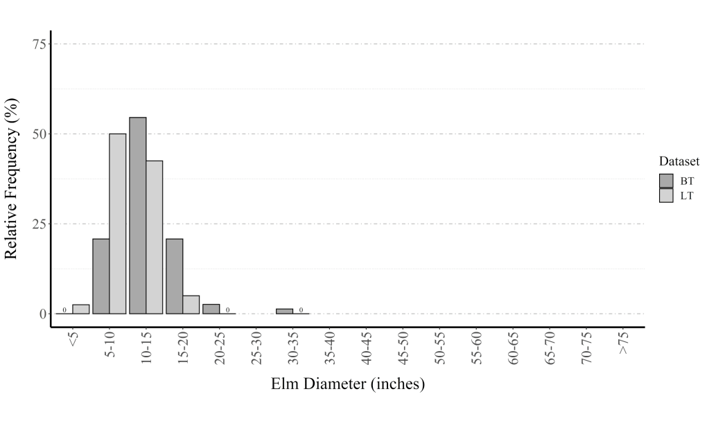
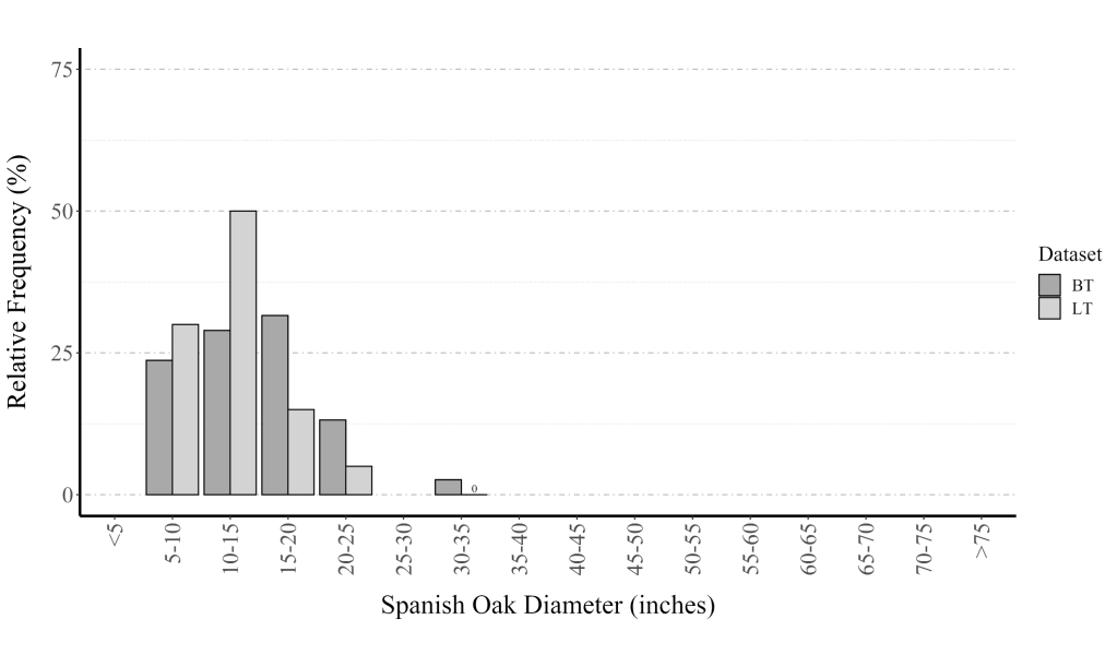
These similarities and differences in species diameters between record types can also be seen in each species diameter distributions. Pine (Fig. 12), white oak (Fig. 13), and black oak’s (Fig. 14) diameter distributions are largely the same between record types, with BT records capturing a slightly higher relative frequency of individuals in the 10–15-inch diameter class for each species.

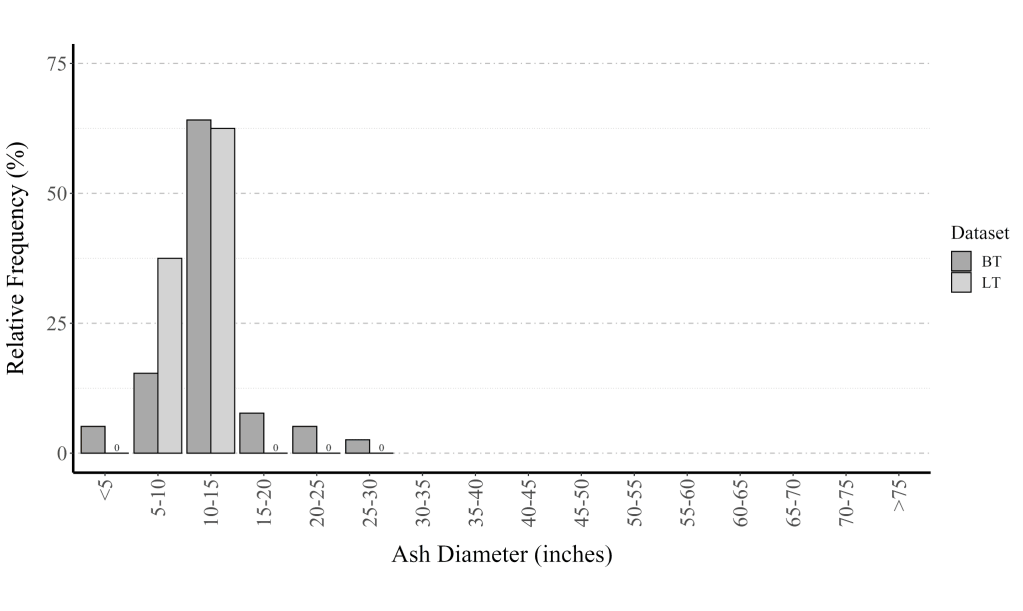
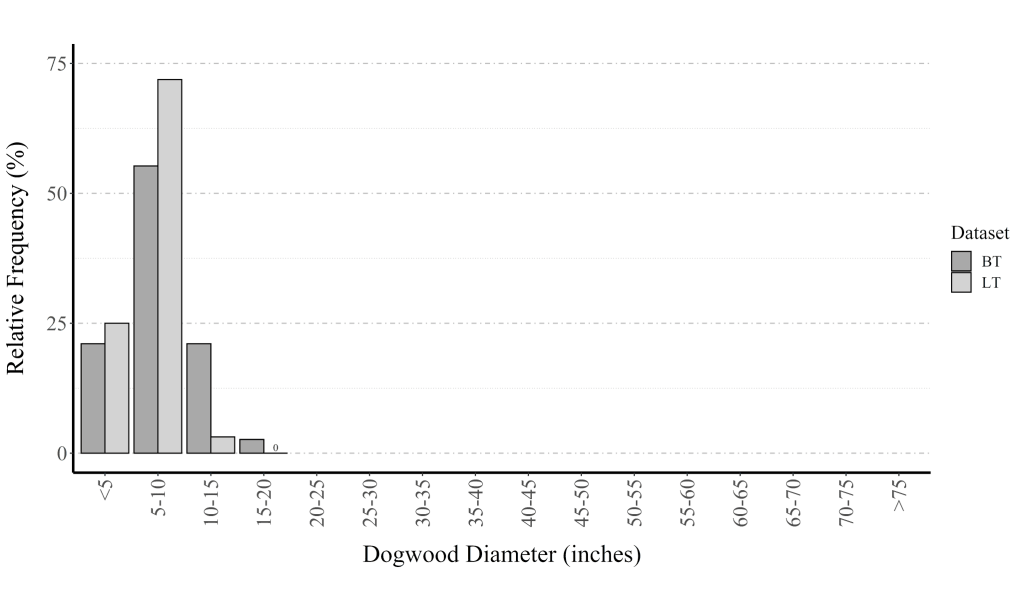
However, Ash (Fig. 15), dogwood (Fig. 16), elm (Fig. 17), and Spanish oak’s (Fig. 18) diameter distributions differ between record types. Ash bearing trees ranged from <5 inches to 25–30 inches, while ash line trees were only recorded in the 5–10 inch and 10–15-inch diameter classes. The relative frequency of ash sampled in the 10–15-inch diameter class was similar in both record types, but ash LTs had a higher frequency of 5–10-inch diameter individuals than ash BTs. Dogwood LTs primarily fell between the <5 inch and 10–15-inch diameter classes, but dogwood BTs recorded a higher relative frequency of individuals in the 10–15-inch diameter class and individuals in the 15–20-inch diameter range. Elm BT and LT diameter distributions were more similar, but >5-inch diameter elms were only recorded in the LT records and 20–25-inch and 30–35-inch size classes were only recorded in the BT records. Spanish oak BT and LT diameter distributions also had a large amount of overlap. However, more 10–15-inch diameter Spanish oaks were recorded as LTs, and several 30–35-inch diameter Spanish oaks were recorded as BTs but not LTs.

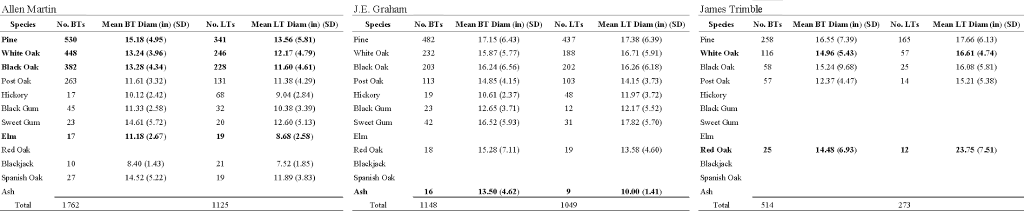
Patterns in species diameter between record types differ by surveyor from the study area wide findings (Table 8). Unlike the cross-ecoregion analysis, the mean diameter of pine (p < 0.001), white oak (p = 0.003), and black oak (p < 0.001) BTs were significantly larger than LTs of the same species in Allen Martin’s surveys. Additionally, white oak (p = 0.042) and red oak (p = 0.002) LTs were significantly larger than BTs of the same species in James Trimble’s surveys, with red oak LTs 9.27 inches larger than red oak BTs on average. Of the species recorded by J.E. Graham with enough records for comparison, only ash had a significant difference in mean diameter between record types with larger BTs (p = 0.011), matching the cross-ecoregion analysis.

Differences in Species Selection

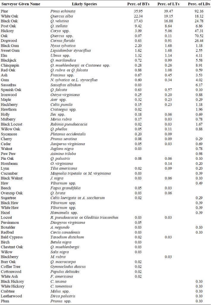
Pine was the most frequently recorded species of all three sampling methods, followed by white oak, black oak, post oak, and hickory (Table 9). Line descriptions more often generalized mentions of oak, instead of listing more specific oak species like BT and LT records did. Bearing trees had the greatest species richness across the entire study area with 48 unique species recorded, followed by LDs species richness of 46 and LTs species richness of 35. BTs captured several understory species missed by LT sampling, including boxelder, cucumber (magnolia), redbud, hawthorn, persimmon, and willow. LDs also captured several understory tree species missed by both BT and LT sampling, including mentions of pawpaw, crabtree, and plum.

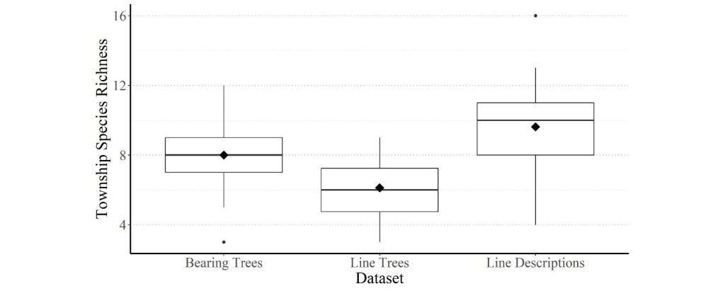
Of the townships collected, 24 townships had BT, LT, and LD records for all 12 township boundary section lines. Allen Martin and James Trimble surveyed a majority of these townships. The records for these townships were used to calculate and compare the average number of species recorded at the township scale using t-tests. Line descriptions had significantly greater township species richness than BTs (p = 0.039) and LTs (p < 0.001), with an average 9.6 species recorded per township (Fig. 19). Bearing trees also had a significantly greater township species richness than LTs, with an average of 8 species recorded per township compared to LTs 6.1 (p = 0.002). Allen Martin recorded the LD outlier of 16 unique species, and James Trimble recorded the BT outlier of 3 unique species.

CHAPTER V: DISCUSSION

Survey Bias in Arkansas’s OME

There is evidence of species and size bias present in GLO surveys conducted in Arkansas’s Ouachita Mountain ecoregion. There are several unique factors influencing the surveying process in Arkansas that may have contributed to this bias in the GLO survey records. First, the collected surveys were completed over a 25-year period. Survey instructions changed over time and were not fully standardized until 1855, after the last collected survey in the ecoregion was completed (White, 1983). In addition to this, the status of Arkansas’s GLO surveying district also changed from 1818 to 1843 (Smith, 2012). From 1815 to 1832, Arkansas was in a surveying district with Illinois and Missouri, and the office for the district was in St. Louis. Because of the large amount of territory under one office and the distance between Arkansas and the district office, surveying progress was slow until Arkansas was given its own survey district and surveyor general, James S. Conway, in late 1832. The slow surveying progress prior to this can be seen in Fig. 5, where 24% of section lines with dated surveys had been completed prior to 1835. These changes in instructions and GLO administration over time could have influenced the collection of the surveys completed during the period Arkansas was in a combined surveying district. Over half of the surveys were completed during an eight-year period from 1835 to 1843 and are less likely to have been influenced by changes in survey instructions and GLO administration. Surveying in Arkansas’s OME was also conducted by 12 different surveyors. (Table 1, Fig. 3). It is likely that each of these surveyors had their own individual preferences for species, tree sizes, and the level of detail of their survey notes, introducing their own unique species and size biases (Liu et al, 2011). This was found for the three surveyors examined individually, who had differing species and size biases present in their BT and LT records (Table 5-6, Table 8).

The influence of survey instructions and surveyor preference can also be seen in the spatial distribution of each of the three types of vegetation records recorded by surveyors. Bearing trees, line trees, and line descriptions had different distributions across the study area. Bearing trees were found across the entire OME (Fig 4.). Line trees were found on 1,412 of the 1,514 of the digitized and mapped section lines (Fig. 5), and line descriptions for true survey divisions were found on 974 section lines (Fig. 6). BTs were required to be surveyed so section corners, the corners of land allotments, could be found later by settlers (White, 1983). These instructions are reflected in the BTs almost total coverage of the digitized and mapped section lines. LTs were not required to be surveyed and had no species or size suggestions in the survey instructions. The only requirement for LTs was that they be trees intersecting the survey line. This is shown in the 102 section lines with no LTs recorded, where surveyors elected not to include LTs in their survey notes. LDs were required to be included in survey records, as the description of the soil condition included in them was needed to determine if the land could be distributed for military bounties (Smith, 2012). However, LDs could be recorded for either the true line or the random line of a section. Random lines were run near true survey divisions to help surveyors orient themselves and determine where the true survey division should be located. As LDs recorded for random lines were not digitized or mapped as a part of this study, the 540 section lines with no mapped LDs likely had them recorded as a part of their random line. 

There was a significant difference in mean species corner-to-tree distances (Table 3). Hickory (p < 0.001), red oak (p = 0.003), dogwood (p < 0.001), and gum’s (p < 0.001) mean corner-to-tree distances were all significantly smaller than all other species (Table 4). The assumption of homogenous forest density across species for entire the study area is likely inaccurate in the OME. This assumption is required for this analysis to detect species bias, rather than differences in forest density. The Ouachitas were frequently subject to fire disturbances during the period the surveys were collected (Fig. 5), which would have created a patchwork landscape of different density forests (Dunbar, 1807; Nuttall, 1821; Featherstonehaugh, 1844; Nowacki & Abrams, 2008). The violation of this assumption means the ANOVA of mean species corner-to-tree distances is instead detecting differences in forest density. It is likely hickory, red oak, dogwood, and gum were instead found more frequently in denser forests overall, rather than being biased against given these factors.

Previous studies have also found significant differences in mean species corner-to-tree distances in GLO surveys in other parts of the United States (Wieh & Dick, 2008; Liu et al., 2011; Williams & Baker, 2010). However, these studies were conducted prior to Kronenfeld’s (2015) publication with the implementation and testing of the relative distance metric. They instead utilized Bourdo (1956) and Delcourt & Delcourt’s (1974) methods. Other studies done prior to Kronenfeld’s (2015) publication found no significant differences in mean species corner-to-tree distances (Dyer, 2001; Delcourt & Delcourt, 1974). The types of forests these studies were conducted in could contribute to these differences in significant and insignificant findings. Wieh & Dick (2008), Liu et al. (2011), and Williams & Baker (2010) study areas were all large and or contained multiple forest types with more diverse forest compositions, likely contributing to their findings of significant differences in mean species corner-to-tree distances. Dyer’s (2001) study area had comparatively more homogenous forest composition, with 40% of bearing trees being white oak, which likely contributed to his insignificant findings. Delcourt & Delcourt (1974) likely did not find significant differences in mean corner-to-tree distance because they analyzed distance-bases species bias by community type, accounting for the different vegetation communities within their study area. Each of the three vegetation communities they examined for BT species bias likely had consistent forest densities for all species within them. Without accounting for differences in forest density across their respective study areas, it is possible these studies were detecting the presence or absence of forest density heterogeneity rather than significant species selection bias. 

We did not find any significant differences in mean species relative distance when examining survey records collectively for the OME (p = 0.109), suggesting the absence of surveyor species selection bias favoring any specific species (Table 3). The relative distance approach addresses the problem of heterogenous forest density across all species for the entire study area. The lack of significant relative distance-based species bias could be contributed to the forest composition of the ecoregion. If pine, white oak, black oak, the dominant species in the OME, were species preferred by surveyors, surveyors would not need to travel greater distances than average to survey them because of their dominance on the landscape. 

Previous studies have suggested that bearing trees located at single-species section corners be removed from analysis because no other species was recorded at that location for surveyors preferentially select over another (Kronenfeld, 2015). Our study area had 2,768 BTs that were excluded from distance-based species bias analyses because they were recorded at section corners with only one species. These BTs were largely pine and oak species (Table 2). This raises questions about the species composition of the OME’s historical forests. It is unlikely that species bias was driving the survey of the large number of pine and oak species recorded. Pine and oak species are consistently the dominant species recorded in all three vegetation record types and across all surveyors examined individually (Table 8-9). While BTs recorded by James Trimble were shown to be biased in favor of pine (Table 6), these preferences were masked by the collective analysis of BT species bias and did not significantly influence overall forest composition captured by BT records (Table 3). Other historical descriptions of the Ouachitas also agree with these findings (Dunbar, 1807; Featherstonhaugh, 1844; Nuttall, 1821). These historical accounts of the Ouachitas forests describe forests as primarily being dominated by pine and oak, lending credence to GLO surveyors in the OME having recorded many section corners of only pine or a single oak species. Overall, it is likely that the dominance of pine and oak species recorded by GLO surveys in the OME was not an effect of species selection bias.

Differences in Bias by Record Type

Size selection bias differed by record type. T-test analyses of mean species diameter between bearing tree and line tree records across the study area revealed that ash, dogwood, and elm surveyed as BTs were significantly larger in diameter than LTs of the same species (Table 7). This suggests that at section corners, surveyors would purposefully select larger individuals of these species to serve as BTs, ignoring smaller ash, dogwood, and elm. This could be attributed to the species being less favorable, given their small contribution to overall forest composition in the BT and LT records (Table 9). These species were likely ignored when preferable species were present and would only be selected if they were of a considerable size for their species. This could also be influencing the smaller mean corner-to-tree distances for these species observed in Table 4. These species likely had to be large, convenient to survey or close, or both large and close to the section corner for surveyors to include them in their records overall. Size selection bias favoring larger ash, dogwood, and elm could also be attributed to the higher density of mesic forests. With many trees in close proximity, larger individuals would likely stand out more to the surveyor. Ash, dogwood, and elm BTs had smaller mean corner-to-tree distances than other, more xeric species, and dogwood had the smallest mean corner-to-tree distance at 4.9 meters, suggesting these species were found in denser forests (Table 3).

Species without significant differences in diameter between record types still showed differences in their diameter distributions (Fig. 11-13). Pine, white oak, and black oak BTs recorded a higher relative frequency of 10–15-inch diameter trees than LTs of the same species. This pattern was also observed in dogwood and elm (Fig. 15-16), which was significantly larger in diameter in BT records than LTs (Table 7). This aligns with surveyor instructions to select the “most permanent and lasting” trees at section corners (White, 1983). This included avoiding the survey of smaller trees, which would have been more likely to die before being relocated and harder to see at a distance. The largest trees were also avoided due to being closer to the end of their lifespan and more likely to be cut first upon the arrival of settlers. The 10–15-inch diameter size class fall into the size range that is neither too small nor too large.

Evidence of both species and size bias differing by record type can be seen in the number of unique species, or species richness, recorded by each type of record. Bearing trees recorded the highest species richness across the study area at 48, and line descriptions recorded the next highest at 46 species. However, line trees only recorded 35 species across the study area. This pattern of low LT species richness can also be seen in the average species richness recorded per township (Fig. 14). LDs recorded an average of 9.6 species per township, significantly higher than BTs 8 species per township (p = 0.039) and LTs 6.1 species per township (p < 0.001). Additionally, both LDs and BTs recorded several understory species missed by LT records (Table 9). These findings suggest surveyors were more selective with what species they surveyed as LTs, ignoring smaller, understory species more frequently. Perhaps because LTs were not a mandatory component of the surveys, surveyor were able to be more selective with their LT survey notes and impose their personal preferences for species and tree size (White, 1983).

Differences in Bias by Surveyor

Distance-based species bias differed between individual surveyors. James Trimble’s surveys showed a significant difference in mean species relative distance, while Allen Martin and J.E. Graham had no significant differences in mean species relative distance (Table 5). Pine in Trimble’s surveys had a significantly larger mean relative distance, while white oak and black gum had a significantly smaller mean relative distance than all other species (Table 6). This suggests Trimble would travel farther distances to survey pine, ignoring closer trees of other species. These findings also suggest Trimble was more likely to survey other species over white oak and black gum. Trimble’s individual species preferences were masked in the study area wide analysis of mean relative distance. Bias should be analyzed on the surveyor level, when possible, to ensure individual surveyor preferences are being accounted for.

There is also evidence of size bias differing between surveyors (Table 5). Pine, white oak, and black oak BTs recorded by Allen Martin were significantly larger in diameter than LTs of the same species. This means Martin preferentially surveyed larger pines, white oaks, and black oaks as BTs. This decision was likely influenced by surveying instructions recommending that surveyors select larger trees for BTs, as they would be likely last long and be more noticeable over a distance (White, 1983). In James Trimble’s surveys, white oak and red oak LTs were significantly larger than BTs of the same species. Red oak LTs in particular were an average of 9.27 inches larger than red oak BTs. The mean diameter of all species analyzed in Trimble surveys were larger in the LT records than BTs, but only the difference in diameter between record types for white oaks and red oaks were statistically significant. However, this trend was not consistent across surveyors. Because line trees were not required to be surveyed, surveyors could choose whether to include them in their records (White, 1983). It is likely that Trimble would only survey line trees if they were large and ignored the smaller trees that intersected the section lines. 

The differences in species diameter by record type observed when analyzing the records collectively differed from Liu et al. (2011), who found LTs of all species were significantly larger than BTs of the same species. Liu et al. (2011) explains their findings by asserting that larger trees would be more likely to be intersected by a random line. However, with strong enough size selection bias towards larger BTs, the effect of larger trees being more likely to intersect the section lines is masked. Liu et al. (2011) also found that surveyors who recorded fewer LTs were more likely to record LTs larger than BTs on average. This was also the case for James Trimble. Of the total trees Trimble recorded, less than 40% were LTs, and his white oak and red oak LTs were significantly larger than BTs of the same species (Table 8). Allen Martin also recorded than 40% LTs out of the total trees he recorded. However, his pine, white oak, black oak, and elm BTs were larger than LTs of the same species. J.E. Graham recorded a more equal number of BTs and LTs, and only his ash BTs were significantly larger in diameter. Perhaps the disparity in the number of BTs and LTs a surveyor records indicates a higher likelihood of size related bias in either BT or LT records.

The average township species richness outliers align with the species bias analysis findings (Fig. 18). Trimble surveyed a township and only recorded 3 unique bearing tree species. In this township, Township 1 North Range 25 West, Trimble recorded 31 pines, 10 white oak, and 7 black oak BTs. The bearing trees James Trimble recorded were found to contain species biased favoring pine and against white oak and black gum (Table 6). This species selection bias could have influenced his survey of this township where he primarily selected pine BTs. Allen Martin surveyed Township 1 North Range 32 West and recorded 16 unique species in the LDs of the township. These included several smaller species such as cherry, magnolia, sassafras, blackjack oak, and “sugartree” (Table 9). Martin’s BTs had no significant species selection bias favoring any particular species (Table 5), and was only biased towards selecting larger pine, white oak, black oak, and elm BTs (Table 8). Martin’s apparent lack of species related bias could have influenced his broader descriptions of the tree species seen along the section lines in this township.

Summary of Species and Size Selection Biases

There is evidence of species and size selection bias in GLO surveys recorded in Arkansas’s Ouachita Mountain ecoregion. The collective analysis of distance-based species bias did not show any significant bias in bearing tree records overall (Table 3). However, the significant differences of mean species relative distances in James Trimble’s bearing tree records indicated he likely favored pine and underrepresented white oak and black gum (Table 5-6). Size biases were also found in BT records when analyzed collectively. Larger ash, dogwood, and elm were preferentially selected as BTs (Table 7). Given their smaller percentage of overall forest composition (Table 9) and smaller mean corner-to-tree distances (Table 3-4), it is likely these species were only surveyed if they were large for their species, close to the section corner and therefore more convenient to survey, or both larger and closer. 

Species and size selection biases differed between record types. Smaller, more mesic understory species were largely excluded from line tree records (Table 9). LTs also collectively recorded less species and less species per township on average (Fig. 19). Line descriptions captured the majority of species ignored by LTs and had the highest number of species recorded per township on average. BTs collectively recorded species richness comparable to LDs, but less species per township on average. This suggests that surveyors were most selective with their choice of species and tree size in LT records, and were less selective when recording BT and LD records. This is likely because LTs survey was completely up to surveyor discretion, while the inclusion of BTs was required (White, 1984). LDs high species richness is likely attributed to their survey only requiring a list of what was seen, rather than specific individuals. Size biases also differed between record types. The collective analysis of size bias showed BT records contain evidence of three species being preferentially surveyed if they were large (Table 7). In the collective analysis, no species were shown to be significantly larger in LT records than BT records. Additionally, a higher relative frequency of mid-sized trees was recorded by BT records compared to LTs records (Fig. 12-18). This is likely an influence of survey instructions recommending surveyors avoid the smallest trees and the largest trees on the landscape (White, 1984).

Lastly, species and size selection biases differed between surveyors. Allen Martin and J.E. Graham’s BT records showed no significant evidence of distance-based species bias, while James Trimble’s BT records showed significantly greater mean relative distance in pine and significantly smaller mean relative distances in white oak and black gum (Table 5-6). The surveyors also differed in their size preferences. Allen Martin surveyed significantly larger diameter pine, white oak, black oak, and elm in his BT records than his LT records (Table 8). J.E. Graham surveyed significantly larger diameter ash in his BT records. On average, James Trimble’s LT records were larger in diameter than his BT records, and white oak and red oak LTs specifically were significantly larger.

While species and size bias is present, the influence of such bias on the survey of dominant forest composition in the OME is minimal. Species and size selection biases did, however, influence the survey of smaller, more mesic species that comprised a smaller percentage of overall forest composition. This could still influence the reconstruction of historical vegetation composition, density, size, and species-site relationships, which would in turn influence landscape management decisions informed by this data. While a smaller component of historical forests, these species are still important to understand and conserve in their historical condition.

Recommendations for the Use of GLO Surveys Considering Bias

Forest Composition

Historical forest composition in Arkansas’s Ouachita Mountain ecoregion would best be reconstructed utilizing line descriptions and bearing tree records in conjunction with one another. LDs captured the highest average species richness per township (Fig. 14) and recorded many smaller, understory species missed by both BT and LT records (Table 9). LDs are best for understanding the total breadth of species present and the presence of rare species. However, there was high variability in the way surveyors recorded species in line descriptions. LDs were often non-specific when mentioning oak, generalizing to the genus rather than mentioning a specific species or group of oaks (Table 9). Surveyors were sometimes very general in their LDs, only mentioning pine and oak, while others were very thorough and noted several tree species in both the timber and undergrowth sections of their LDs. This high degree of variability in the recording of LDs was also noted by Batek et al. (1999) and Manies & Mladenoff (2000) in the GLO survey notes they examined. LDs recorded for true lines also had a limited distribution, as surveys split their LD notes between true and random lines (Fig. 6). Because of these limitations, bearing tree records would be best utilized for reconstructing the dominant forest composition in the OME. BT records allow for a quantitative description of species composition and examination of the dominance of particular species. The majority of BT records were specific when identifying species rather than generalizing to a genus (Table 9). BTs recorded along the same line as LDs can be used to clarify generalized LD records of oak. In areas outside the OME, the species richness and the variability of surveyor records should be compared for all three record types. The record type with greater species richness and lower variability how surveyors described species are best applied to reconstructions of historical forest composition. 

Forest Density

Historical forest density can be reconstructed using bearing trees recorded by surveyors who did not show significant species or size biases in their BT records. The study area wide analysis showed no significant differences in relative distance (ƒ = 1.5, p = 0.109) (Table 3). However, the analysis of all BT records together masked individual surveyor species biases. James Trimble’s surveys showed significant differences in relative distance by species (ƒ = 2.7, p = 0.013). Trimble’s BT records were found to be biased in favor of pine and against white oak and black gum. Trimble was likely traveling farther from the section corner in order to survey pine, ignoring closer trees of other species. This could cause forest density reconstructions based on Trimble’s BT records would show lower overall densities than what was present. Size-related bias could also influence reconstructions of density. Although Allen Martin’s BT records did not have significant differences in mean relative distance between species (ƒ = 0.8, p = 0.643), Martin’s BT records were biased towards the selection of larger pine, white oak, black oak, and elm (Table 8). Forest density reconstructions based on Martin’s BT records would reflect the density of the most mature trees on the landscape rather than the density of the forest as a whole. Additionally, the size biased pine, white oak, and black oak BTs are the dominant species of the OME’s historical forests (Table 9). The prevalence of these species would likely increase the influence of the size selection bias on density reconstructions.

Of the surveyors examined individually in Arkansas’s OME, J.E. Graham’s BT records would be able to be utilized for reconstructing historical forest density. Graham’s BTs showed no significant differences in relative distance between species (ƒ = 1.4, p = 0.170) (Table 5). Additionally, Graham’s BT records only showed significant size bias favoring the selection of larger ash (Table 8), which comprises a small percentage of overall forest composition (Table 9). The low species and size bias in Graham’s records make them ideal for reconstructing forest density. In areas outside the OME, the species and size selection bias in BT records should be examined on the surveyor level before utilizing their surveys to reconstruct historical forest density.

Species Diameter Distributions

Diameter distributions can be reconstructed using LT or BT records depending on the size bias present at the surveyor level. In the study area wide analysis, and within Allen Martin and J.E. Graham’s surveys specifically, several species were significantly larger in BT records than in LT records (Table 7-8). Additionally, BTs captured a higher relative frequency of 10–15-inch diameter individuals than LTs (Fig. 11-13, 15-16), as survey instructions recommended that surveyors select BTs that were “the size and kinds of trees which experience teaches will be the most permanent and lasting.” (White, 1983). However, these patterns of bias in BT size selection are not consistent for all surveyors. James Trimble’s LT records showed bias towards larger diameter white oak and red oak (Table 8). Overall, LTs are better for reconstructing diameter distributions in the OME, except for surveys recorded by James Trimble. Size bias should be assessed on the surveyor scale, and BTs should be applied instead LTs for diameter distribution reconstructions when a surveyor shows evidence of size bias favoring the selection of larger LTs. In areas outside the OME, by surveyor comparisons of BT and LT size by species should be made to determine the presence of such bias. Comparisons of species diameter distributions by record type should also be made to see if survey instructions influenced the selection of mid-sized trees in BT records. After drawing these comparisons, the determination of which of the two record types are best applied for each surveyor can be made.

Species-site Relationships

Bearing tree and line tree records are better utilized to reconstruct species-site relationship than line descriptions in the OME. LDs included species seen over half-mile or one-mile segments. Most section lines only had one LD for the entire one-mile section line, including species seen along the entire segment. The shifts in site conditions over these distances are likely too broad to connect species to environmental variables in a meaningful way. However, Tulowiecki (2014) was able to successfully reconstruct species-site relationships using LDs in his study area in Chautauqua County, New York. Chautauqua County was surveyed by the Holland Land Company, who applied the PLSS like GLO surveys but had different surveying instructions. LDs in Holland Land Company surveys covered smaller segments of the section line than LDs in GLO surveys in the OME. With less variation in environmental conditions over the smaller segments, species recorded in LDs were more accurately associated with topographic and edaphic variables. This allowed Tulowiecki (2014) to establish species-site relationships using LDs and utilize these established relationships to model early Euro-American settlement forest composition and structure.

Size selection bias found within bearing and line tree records could potentially influence the reconstruction of historical species-site relationships. Tree size is both a function of age and the conditions in which the tree is found. The larger trees selected by surveyors could be found on more productive sites than the smaller trees surrounding them which were excluded. This could cause species-site relationship reconstruction to be biased towards more productive sites, rather than the full range of conditions the species were found in historically. In the OME, species-site relationships should be reconstructed with line tree records, expect for surveyors who showed size bias in their LT records like James Trimble. In areas outside the OME, size bias in BT and LT records should be evaluated for the area as a whole and by surveyor. The record type with the least size bias for each surveyor should be applied for reconstructing species-site relationships to avoid the potential influence of size bias on the results of the reconstructions.

CHAPTER VI: CONCLUSION

Prior to Euro-American settlement, the Arkansas’s Ouachita Mountains were found to be dominated by shortleaf pine (Pinus echinata) and oak (Quercus spp.) woodlands. These low density, fire-adapted woodlands provide habitat for several of Arkansas’s threatened species. Today these woodland habitats are in decline due to the removal of the wildfire disturbances that maintained their unique composition and structure. It is for these reasons that shortleaf pine-oak woodlands are a focus of conservation and restoration in Arkansas. Information is needed on the historical fine-scale distribution, composition, and structure of these fire-adapted habitats in Arkansas’s Ouachita Mountain ecoregion to help guide landscape management efforts.

General Land Office surveys are a resource of detailed pre- and early settlement period forest distribution, density, and composition (Batek et al. 1999; Foti & Glenn, 1991; Hanberry et al., 2012; Tulowiecki, 2014; Wang, 2005). However, these surveys are not free from species and size selection bias introduced by individual surveyor preferences and the surveyor instructions themselves. This creates a skewed view of pre- and early-settlement vegetation with species and size selection biases that differ spatially, by deputy surveyor, and by the vegetation record type (Bourdo, 1956; Wang, 2005; White, 1983). It is necessary to evaluate the unique selection biases present in GLO surveys, as bias could influence reconstructions of historical forest composition, density, species diameter distributions, and species-site relationships. 

This study analyzed the species and size bias in GLO bearing tree, line tree, and line description records for Arkansas’s Ouachita Mountain ecoregion and provided recommendations for using these records for historical vegetation reconstructions given the observed bias. Evidence of bias was found within GLO surveys conducted in Arkansas’s OME. The changes in surveyor instructions and GLO administration over the early survey collection period, and the individual preferences for species, tree sizes, and survey record detail of the 12 different surveyors who conducted the surveys are likely to have contributed to the species and size biases found. The species and size biases observed were also found to differ between the types of vegetation data recorded and between surveyors. Individual surveyor species and size bias was masked when analyzing all surveyor records collectively. Bias analyses should be conducted at the surveyor level, in addition to study area wide analyses, to detect individual surveyor preferences for species or tree sizes. 

With 70% of the GLO surveys for Arkansas’s OME digitized, mapped, and analyzed for bias, future research could be dedicated to the reconstruction of historical forest composition, density, species diameter distribution in the ecoregion. The specific locations of each species recorded in both BT and LT records could be associated with environmental site conditions to also reconstruct species-site relationships. These species-site relationships could then be used to model historical species distributions across the OME, instead of just along survey divisions. These species distributions reconstructions could also be compared to the modern forests of the OME to see the extent of landscape change since the early 1800s. Additionally, future research could also complete the full survey collection, digitization, and mapping of the ecoregion. This would allow for the examination of species and size selection biases of additional surveyors in the OME. This would further explore the influence of Arkansas’s GLO history on the collection of these surveys and their species and size biases in the state. 

REFERENCES

ABBYY. (2020). FineReader PDF 15 Standard (Build 15.0.117.9681). ABBYY Production LLC. https://pdf.abbyy.com/.

Abrams, M. D., Nowacki, G. J., & Hanberry, B. B. (2022). Oak forests and woodlands as Indigenous landscapes in the Eastern United States. The Journal of the Torrey Botanical Society.

Arkansas Division of Land Surveys & Arkansas GIS Office. (2022). GLO Map 2.3. https://agio.maps.arcgis.com/apps/webappviewer/index.html?id=a12855ed847c4c268b563f261efd11ec.

Batek, M. J., Rebertus, A. J., Schroeder, W. A., Haithcoat, T. L., Compas, E., & Guyette, R. P. (1999). Reconstruction of early nineteenth‐century vegetation and fire regimes in the Missouri Ozarks. Journal of Biogeography, 26(2), 397-412.

Black, B. A., Ruffner, C. M., & Abrams, M. D. (2006). Native American influences on the forest composition of the Allegheny Plateau, northwest Pennsylvania. Canadian Journal of Forest Research, 36(5), 1266-1275.

Bolliger, J., Schulte, L. A., Burrows, S. N., Sickley, T. A., & Mladenoff, D. J. (2004). Assessing Ecological Restoration Potentials of Wisconsin (U.S.A.). Restoration Ecology, 12(1), 124-142.

Bourdo, E. A. (1956). A review of the General Land Office survey and of its use in quantitative studies of former forests. Ecology, 37(4), 754-768.

Bragg. D.C. (2003). Natural presettlement features of the Ashley County, Arkansas area. American Midland Naturalist, 149(1), 1-20.

— (2004a). General Land Office Surveys as a Source for Arkansas History, The Example of Ashley County. The Arkansas Historical Quarterly, 63(2), 166-184.

—. (2004b). Patterns of Oak Dominance in the Eastern Ouachita Mountains Suggested by Early Records. Gen. Tech. Rep. SRS-73. Asheville, NC: U.S. Department of Agriculture, Forest Service, Southern Research Station, 57-61.

Bragg, D. C., & Webb, T. (2014). ” As False as the Black Prince of Hades”: Resurveying in Arkansas, 1849-1859. The Arkansas Historical Quarterly, 73(3), 268-292.

Breiman, L. (2001). Random forests. Machine learning, 45(1), 5-32.

Brooks, R. L. (2010). Analyzing the Arkansas River Caddoan Cultural Landscape. Caddo Archaeology Journal, 20, 35-55.

Delcourt, H. R., & Delcourt, P. A. (1974). Primeval magnolia‐holly‐beech climax in Louisiana. Ecology, 55(3), 638-644.

Dunbar, W. (1807). Travels in the Interior Parts of America; Communicating Discoveries Made in Exploring the Missouri, Red River and Washita, by Captains Lewis and Clark, Doctor Sibley, and Mr. Dunbar; with a Statistical account of the Countries Adjacent. As Laid Before the Senate, by the President of the United States. In February, 1806, and Never Before Published in Great Britain. Richard Phillips.

Dyer, J. M. (2001). Using witness trees to assess forest change in southeastern Ohio. Canadian Journal of Forest Research, 31(10), 1708-1718.

Esri. (2021). ArcGIS Pro (2.8.2). ESRI Inc. https://www.esri.com/en-us/arcgis/products/arcgis-pro/overview.

Evans, J. S., Murphy, M. A., Holden, Z. A., & Cushman, S. A. (2011). Modeling species distribution and change using random forest. In Predictive species and habitat modeling in landscape ecology (pp. 139-159). Springer.

Featherstonhaugh, G. W. (1844). Excursion through the slave States: from Washington on the Potomac, to the frontier of Mexico; with sketches of popular manners and geological notices. Harper. 

FGDC Cadastral Subcommittee & Arkansas GIS Office. (2014). PLSS: Intersected, BLM [Vector data file]. Arkansas GIS Office. https://gis.arkansas.gov/product/plss-intersected-blm/.

Foti, T. L. (2022). Hello & GLO Stuff. In W. Flatley (Ed.), (E-mail communication ed.).

Foti, T. L., & Glenn, S. M. (1991). The Ouachita Mountain landscape at the time of settlement. 49–65. Proceedings of the conference on restoration of old-growth forests in the interior highlands of Arkansas and Oklahoma Arkansas, USA Ouachita National Forest and Winrock International Institute for Agricultural Development.

Grimm, E. C. (1984). Fire and other factors controlling the Big Woods vegetation of Minnesota in the mid‐nineteenth century. Ecological Monographs, 54(3), 291-311.

Finley, R. W. (1951). The original vegetation cover of Wisconsin (Doctoral dissertation).

Hanberry, B. B., Dey, D. C., & He, H. S. (2012). Regime shifts and weakened environmental gradients in open oak and pine ecosystems. PLoS One, 7(7), e41337.

He, H. S., Dey, D. C., Fan, X., Hooten, M. B., Kabrick, J. M., Wikle, C. K., & Fan, Z. (2007). Mapping pre-European settlement vegetation at fine resolutions using a hierarchical Bayesian model and GIS. Plant Ecology, 191(1), 85-94.

Hedrick, L. D., Bukenhofer, G. A., Montague, W. G., Pell, W. F., & Guldin, J. M. (2007). Shortleaf pine-bluestem restoration in the Ouachita National Forest. In: Shortleaf pine restoration and ecology in the Ozarks: proceedings of a symposium: 206-213.

Jawarneh, R. N., & Julian, J. P. (2012). Development of an accurate fine-resolution land cover timeline: Little Rock, Arkansas, USA (1857–2006). Applied Geography, 35(1-2), 104-113.

Kronenfeld, B. J. (2015). Validating the historical record: a relative distance test and correction formula for selection bias in presettlement land surveys. Ecography, 38(1), 41-53.

Kronenfeld, B. J., & Wang, Y.-C. (2007). Accounting for surveyor inconsistency and bias in estimation of tree density from presettlement land survey records. Canadian Journal of Forest Research, 37(11), 2365-2379.

Larsen, C. P., Tulowiecki, S. J., Wang, Y. C., & Trgovac, A. B. (2015). Predicting historic forest composition using species lists in presettlement land survey records, western New York. Applied Vegetation Science, 18(3), 481-492.

Liu, F., Mladenoff, D. J., Keuler, N. S., & Moore, L. S. (2011). Broadscale variability in tree data of the historical Public Land Survey and its consequences for ecological studies. Ecological Monographs, 81(2), 259-275.

Lorimer, C. G. (1977). The presettlement forest and natural disturbance cycle of northeastern Maine. Ecology, 58(1), 139-148.

Lutz, H. J. (1930). Original forest composition in northwestern Pennsylvania as indicated by early land survey notes. Journal of Forestry, 28(8), 1098-1103.

Manies, K. L., & Mladenoff, D. J. (2000). Testing methods to produce landscape-scale presettlement vegetation maps from the US public land survey records. Landscape Ecology, 15(8), 741-754.

Masters, R. E. (2007). The importance of shortleaf pine for wildlife and diversity in mixed oak-pine forests and in pine-grassland woodlands. Shortleaf pine restoration and ecology in the Ozarks: proceedings of a symposium.

Nowacki, G. J., & Abrams, M. D. (2008). The demise of fire and “mesophication” of forests in the eastern United States. BioScience, 58(2), 123-138.

Nuttall, T. (1821). A journal of travels into Arkansas Territory, during the year 1819 with occasional observations on the manners of the aborigines. Thos. H. Palmer. 296.

Ogle, J., Witsell, T., & Gentry, J. L. (2020). Trees, shrubs, and woody vines of Arkansas. Ozark Society Foundation.

Olsen, L. M., Dale, V. H., & Foster, T. (2007). Landscape patterns as indicators of ecological change at Fort Benning, Georgia, USA. Landscape and urban planning, 79(2), 137-149.

Ouachita Mountains Ecoregional Assessment Team. (2003). Ouachita Mountains ecoregional assessment. Arkansas Field Office and Oklahoma Field Office.

R Core Team. (2021). R: A language and environment for statistical computing. R Foundation for Statistical Computing, Vienna, Austria. https://www.R-project.org/.

Schoolcraft, H. R. (1819). A view of the lead mines of Missouri: including some observation on the mineralogy, geology, geography, antiquities, soil, climate, population, and productions in Missouri and Arkansaw, and other sections of the western country. Charles Wiley & Co. 299.

Schulte, L. A., & Mladenoff, D. J. (2001). The original US public land survey records: their use and limitations in reconstructing presettlement vegetation. Journal of Forestry, 99(10), 5-10.

Schulte, L. A., Mladenoff, D. J., & Nordheim, E. V. (2002). Quantitative classification of a historic northern Wisconsin (USA) landscape: mapping forests at regional scales. Canadian Journal of Forest Research, 32(9), 1616-1638.

Smith, D. A. (2012). Preparing the Arkansas Wilderness for Settlement: Public Land Survey Administration, 1803-1836. The Arkansas Historical Quarterly, 71(4), 381-406.

Strausberg, S. F. & Hough, W. A. (1997). The Ouachita and Ozark-St. Francis National Forests, a History of the Lands and USDA Forest Service Tenure (Vol. 121). US Department of Agriculture, Forest Service, Southern Research Station.

Tulowiecki, S. J. (2014). Using vegetation data within presettlement land survey records for species distribution modeling: A tale of two datasets. Ecological modelling, 291, 109-120.

—. (2020). Modeling the historical distribution of American chestnut (Castanea dentata) for potential restoration in western New York State, US. Forest Ecology and Management, 462, 118003.

Tulowiecki, S. J., & Larsen, C. P. (2015). Native American impact on past forest composition inferred from species distribution models, Chautauqua County, New York. Ecological Monographs, 85(4), 557-581.

U.S. Environmental Protection Agency. (2010). Level III Ecoregions of Arkansas [Vector data file]. U.S. EPA Office of Research & Development (ORD) & National Health and Environmental Effects Research Laboratory (NHEERL). https://www.epa.gov/eco-research/ecoregion-download-files-state-region-6.

U.S. Forest Service. (2005). Revised Land and Resource Management Plan, Ouachita National Forest, Arkansas and Oklahoma. https://www.fs.usda.gov/Internet/FSE_DOCUMENTS/fsm9_039609.pdf

—. (2017a). FY 2017 Annual Monitoring Report of the Land and Resource Management Plan Ouachita National Forest. https://www.fs.usda.gov/Internet/FSE_DOCUMENTS/fseprd594873.pdf

—. (2017b). Ouachita National Forest Monitoring Activities. https://www.fs.usda.gov/Internet/FSE_DOCUMENTS/fseprd505030.pdf

U.S. Geological Survey. (2022). National Hydrography Dataset (ver. USGS USGS National Hydrography Dataset Best Resolution (NHD) – Arkansas (published 20221013)). https://www.usgs.gov/the-national-map-data-delivery.

U.S. Geological Survey. (2020). 3D Elevation Program 30-Meter Resolution Digital Elevation Model (published 20201002). https://www.usgs.gov/the-national-map-data-delivery.

Wang, Y.-C. (2005). Presettlement land survey records of vegetation: geographic characteristics, quality and modes of analysis. Progress in Physical Geography, 29(4), 568-598.

—. (2007). Spatial patterns and vegetation–site relationships of the presettlement forests in western New York, USA. Journal of Biogeography, 34(3), 500-513.

Weih Jr, R. C., & Dick, A. (2008). Historical forest landscape changes in the Buffalo River sub-basin in Arkansas. Journal of the Arkansas Academy of Science, 62(1), 115-124.

White, C. A. (1983). A history of the rectangular survey system. US Department of the Interior, Bureau of Land Management.

Williams, M. A., & Baker, W. L. (2010). Bias and error in using survey records for ponderosa pine landscape restoration. Journal of Biogeography, 37(4), 707-721.